Download
1 / 62
620 likes | 725 Views
Search for Charged Higgs in t t Decay Products at CDF II. Ricardo Eusebi University of Rochester, CDF. Outline : Introduction and Motivation Tevatron and CDF II Analysis Technique Results The future Summary. Introduction and Motivation. Fundamental Questions. Intro.

E N D
Search for Charged Higgs in tt Decay Products at CDF II Ricardo Eusebi University of Rochester, CDF Outline : Introduction and Motivation Tevatron and CDF II Analysis Technique Results The future Summary
Fundamental Questions Intro • Fundamental questions of Contemporary Physics • What is dark energy ? Dark matter ? • What’s the deal with neutrinos ? • Why so many particles ? What’s the reason for their masses ? • Are there other symmetries ? • Are all the forces related at some high energy ? • Standard Model of particles and fields (SM) • Electroweak symmetry (EWS). Massless particles predicted. • The Higgs field breaks symmetry (EWSB) generating mass. Predicts h0(SM). • But we can’t find the h0. Maybe another mechanism in place ? New particles ? • The unknown mechanism of EWSB is a key aspect to help answer some of the fundamental questions of the Universe. Ricardo Eusebi - Fermilab Interview
Electroweak Symmetry Breaking Intro • Top • Large mass suggest it plays an important role • Fermion to which coupling to Higgs is most important, yt=Mt/v ≈ 1. • Standard Model (SM) : 1 Higgs doublet • EWSB One Higgs boson, h0(SM) • Decays to bb , tt, etc. • Excluded up to ~114 GeV • Natural Next step : Models with 2 Higgs Doublets (2HDM) • EWSB 5 Higgs bosons (h0,H0,A,H±) • h0, H0 bb, tt, gg, W+W-, ZZ, cc • A bb, tt, gg, Zh0, tt • H+tb, tn, cs, W+h0, W+A • h0 excluded up to ~95 GeV • What can be said about H±? Ricardo Eusebi - Fermilab Interview
Charged Higgs Production at the Tevatron Intro • Direct C.H. Production • Tevatron : qqH+H- • Very small production rate • Signature hard to distinguish • Indirect C.H. Production • Tevatron : top associated • If mtop>mH+mb from tt decays • If mtop<mH with associated top • Maybe Large production rates • Clean signature Ricardo Eusebi - Fermilab Interview
Importance of top and higgs in EWSB • H± might be produced with top Where can we study this ? Tevatron and CDF II
The CDF II Detector at the Tevatron • Quadrant of the CDF II detector section view • Sampling Calorimeters • Iron/scin (HAD) • Pb/scin (EM) • Coverage |h|<3.6 HAD • Tracking system • Solenoid 1.4 Tesla • Central Outer Tracker Drift wires • Silicon Detectors determination of secondary vertexes HAD EM HAD • CDF II • Good determination of angles and energies for e’s, m’s and jets. • Calculation of MET EM Ricardo Eusebi - Fermilab Interview
H± might be produced with top • Tops are produced at the Tevatron How can we study it ? Analysis Technique
Anal. Ricardo Eusebi - Fermilab Interview
W- jets e W+ e jets S/B~0.04 S/B~1 all-jets lepton+jets S/B~1 S/B~3 lepton+jets dilepton Top Pair SM Signatures Anal. • In the SM, BR(tW+b) >0.99 @95%CL • Final state is given by W+ and W- decays • All Hadronic channel (tt bqq′bqq) • Large BR • Small S/B • Lepton (e,m) + Jets channel (tt blbqq′) • Second large BR • Good S/B • overconstrained kinematics • Dilepton channel : (tt blbl) • BR is ¼ of L+Jets • cleanest channel • underconstrained kinematics • Lepton + Hadronic Tau channel(tt blvbthn ) • Very small BR • S/B~1 • Production cross section measured in all these channels Lep.+Tau Lep.+Tau Ricardo Eusebi - Fermilab Interview
Top Pair Search Channels Anal. • Take advantage of existent cross section analyses • Lepton+Jets (1, and 2 or more tags) hep-ex/0409029, 0410041 • Lepton+Tau To be published • Dilepton Phys. Rev. Lett. 93, 142001 (2004) • Lepton+Jets(1) sample requires: • Isolated lepton (e,m) with ET>20 GeV • MET>20 GeV • at least 4 jets with ET>15 GeV • One or more b-tagged jets • Lepton+Tau sample requires: • Isolated lepton (e,m) with ET>20 GeV • MET>20 GeV • 1 jet ET>15 GeV, other with ET>25 GeV • Hadronically decaying tau, PT>15 • We will not use them directly as they are. Small changes will be needed. • Lepton+Jets(2) sample requires: • Isolated lepton (e,m) with ET>20 GeV • MET>20 GeV • at least 4 jets with ET>15 GeV • Two or more b-tagged jets • Dilepton sample requires : • Two leptons (ee, μμ, eμ) ET>20 GeV • MET>20 GeV • at least two jets with ET>15 GeV. Ricardo Eusebi - Fermilab Interview
Top-associated Higgs Boson Signatures Anal. • Higgs Boson decays : • h0, H0 bb, tt, gg, W+W-, ZZ, cc • A bb, tt, gg, Zh0, tt • H+tb, tn, cs, W+h0, W+A • If H± is present, what do we expect ? • If H+tn, • Lepton+Tau sample may show excess w.r.t. SM expectations. • Dilepton and Lepton+Jets show a deficit • If H+cs, • All channels would show a deficit. • Similar consideration for other H+ decays. • Thepresenceof an H± would affect the relative number of events in each top decay channel, according to its decay. Search strategy Look at the relative rates of events in different tt decay channels Ricardo Eusebi - Fermilab Interview
Anal. Ricardo Eusebi - Fermilab Interview
Charged Higgs Decays Considered Anal. • Assume that top decays either to W+b or H+b • tW+b • tH+b • Assume that the Higgs decay only as follows : • H+cs • H+tn • H+t*B • H+W+h0 • We further consider the h0 decays to bb • h0bb • Summary : For each top quark we consider 5 possible decays modes B1. tW+b B2. tH+bcsb B3. tH+btnb B4. tH+bt*Bb B5. tH+bW+h0bW+bbb The BR to each (Bi) can be predicted from these 5 indep. BR’s The Narrow Width Approximation (NWA) is implicit. Ricardo Eusebi - Fermilab Interview
Number of Expected Events Anal. • Dilepton, lepton+jets ≡1 and ≥2 tags, lepton+tau XS analyses (XSA) Includes Luminosity Ricardo Eusebi - Fermilab Interview
Number of Expected Events, Nback Anal. • Dilepton, lepton+jets ≡1 and ≥2 tags, lepton+tau XS analyses (XSA) Taken from the cross section measurement • Assume non-SM backgrounds to be negligible • ppWh0(MSSM) < s(Wh0SM) < 0.2 pb • ppZh0(MSSM) < s(Zh0SM) < 0.1 pb • ppH+H- • ppW+H- • H+ production via decay of heavy SUSY particles. Ignored here. Ricardo Eusebi - Fermilab Interview
Number of Expected Events, s Anal. • Dilepton, lepton+jets ≡1 and ≥2 tags, lepton+tau XS analyses (XSA) Use the theoretical production cross section stheo=(6.7±0.7)pb, hep-ph0303085 • Assume that introduction of the Higgs sector do not change the production mechanism. Ricardo Eusebi - Fermilab Interview
Number of Expected Events, Bi’s Anal. • Dilepton, lepton+jets ≡1 and ≥2 tags, lepton+tau XS analyses (XSA) Bi (Bj) : Branching fractions of top (anti-top) decay mode Total efficiency calculated from top and anti-top branching ratio decay modes. • Recall that the Bi’s are calculated assuming the Narrow Width Approximation is valid. The analysis is limited to regions in which the widths of top and Higgs are each below 15 GeV. Ricardo Eusebi - Fermilab Interview
Number of Expected Events, ei,j XSA Anal. • Dilepton, lepton+jets ≡1 and ≥2 tags, lepton+tau XS analyses (XSA) Mode-specific efficiency Mode-specific efficiency determined given (Gtop, GHiggs, mH±, mh0) • It is the efficiency of the tt event with modes i, j given the mass of the charged Higgs and the mass of the neutral Higgs h0. • It takes into account corrections due to large width of the top and Higgs. Let’s look at ei,j XSA in more detail Ricardo Eusebi - Fermilab Interview
Number of Expected Events, ei,jXSA Anal. ei,jXSA(Gtop,GHiggs,mH±,mh0)is written as (dropping the i,j subindex): Known. Includes eff’s and scale factors from trigger, lepton, etc. See respective papers. Obtained running the XSA selection code over the datasets with proper masses. (Dataset contains the 15 different channels.) Ricardo Eusebi - Fermilab Interview
Problem : Pythia lacks the ME of H+t*bWbb Anal. • Used to have it. Got drop sometime between 2000 and 2004. • Talked to Mrenna about the possibility of adding the decay. • In this analysis we took the ME from PRL 80, 1162 (1998), and place it into a custom madePythia. • The MSSM parameters do not deform the topology of the decay, just scale it changing the BR. • Thoroughly checked! • First check that the eff in the channels w/o a H+->t*b decay does not change. • Then check that the density of points in the Dalitz plot agrees with the ME. • Finally integrate the Dalitz plot and cross check that it gives the same BR as predicted by PRL 80,1162. Overall small change in efficiencies w.r.t. 3-body decay Ricardo Eusebi - Fermilab Interview
Number of Expected Events, ei,jXSA Anal. ei,jXSA(Gtop,GHiggs,mH±,mh0)is written as (dropping the i,j subindex): Known. Includes eff’s and scale factors from trigger, lepton, etc. See respective papers. Obtained running the XSA selection code over the datasets with proper masses. (Dataset contains the 15 different channels.) Ricardo Eusebi - Fermilab Interview
Width Corrections, qualitatively Datasets interpolation Anal. • Different widths different mass distributions. Generate Datasets with -- mTop =165,175,185 -- narrow width. Calculate the efficiencies and interpolate between the points. Width-corrected efficiency integral of e(mTop) weighted by the mass distribution Top mass = 175 GeV Gtop = 10 GeV e(mtop) • Note : If efficiency is linear, and mass spectrum symmetrical, the correction would be null. Ricardo Eusebi - Fermilab Interview
Wt(175,wT) for diff wT Width Corrections, quantitatively Anal. Width correction taken into account when doing : After corrections Width corrections are very small, although we still take them into account. Ricardo Eusebi - Fermilab Interview
from MC from XS meas. stheo=(6.7±0.7)pb (hep-ph 0303085) Branching fractions of each decay mode Number of Expected Events : Summary Anal. • Dilepton, lepton+jets ≡1 and ≥2 tags, lepton+tau XS analyses (XSA) • 9 quantities needed to fully determine ett,XSA • 5 BR’s, Gtop,GHiggs, mH± and mh0 Ricardo Eusebi - Fermilab Interview
Anal. Ricardo Eusebi - Fermilab Interview
Methodology : NObsv -mexp comparison Anal. • Comparison by means of Likelihood • where the were defined previously • calculate the likelihood by using MC integration Number of candidates in each XS Relevant parameter set from which the 9 quantities can be calculated Product of Poisson's XS’s must be exclusive! Correlations between XS’s fully taken into account! Ricardo Eusebi - Fermilab Interview
Removal of Overlap Between XS’ Anal. • Separate the lepton+jets into exactly 1 tag and 2 or more tags • Signal Overlap between lepton+jets and dilepton ? • No. Lepton+jets has a dilepton veto • Signal Overlap between XSA and lepton+tau, given by • FXSA # events passing both XSA and lepton+tau / # events passing XSA ~1% for SM up to 15% if Higgs is present • Strategy : • Implement a lepton+tau veto cut in the lepton+jets and dilepton XS’s. • Recalculate signal (and background) efficiencies Ricardo Eusebi - Fermilab Interview
R. of Overlap, New Background Estimates Anal. • Background Overlap between LTauh and rest, given by FXSA • FXSA # events passing both XSA and Lepton+Tau / # events passing XSA The Lepton+tau veto cut leaves the backgrounds essentially unchanged ! Ricardo Eusebi - Fermilab Interview
Anal. Ricardo Eusebi - Fermilab Interview
Limits on Model Anal. • We use Bayesian statistics • Parameter we would like to set limits on, a • Posterior probability density as a function of a • L is the likelihood • p(a) is the prior in a. • Limits in a set by integrating the posterior over the maximum density region until obtaining 0.95 Ricardo Eusebi - Fermilab Interview
Relative rates of events in different channels can set limits on H± models • Can set limits on any model that predicts the 9 quantities. What models to use?, what are the results ? Results
Results : MSSM Res. • Several parameterizations of MSSM • General MSSM : • intergenerational mixing. • Complex phases. • 105 input parameters in addition to the SM ones. • Phenomenological MSSM : • Soft SUSY breaking parameters are real. No new sources of CP violation. • Matrices for sfermions and trilinear couplings are diagonal. No FCNC at tree level. • Masses and trilinear couplings of 1st and 2nd generation are equal. • 22 input parameters. Down to 14 if only third generation needed. • GUT-constrained MSSM (mSUGRA) • Unification of gaugino masses. • Universal scalar masses. • Universal trilinear coupling. • 4 and a half parameters. • We use the Phenomenological MSSM (pMSSM), with 14 parameters. • Use different sets of pMSSM parameters (or benchmark scenarios) Ricardo Eusebi - Fermilab Interview
Results : MSSM , Choice of Benchmarks Res. • LEP benchmarks revisited • Maximal and minimal stop mixing scenarios. • Maximize and minimize the mass of the h0 as a function of tan(b). • All parameters except At fixed. At is chosen so as to maximize or minimize mh0 • The decay H+ W+h0 larger around tan(b)≈1 • G(Htn,cs,t*b) is bigger at lower and higher tan(b) values • Maximization or minimization of the h0 mass useful at tan(b)≈1 Ricardo Eusebi - Fermilab Interview
m=-500 GeV m=+500 GeV Results : MSSM , Choice of Benchmarks Res. • BR(tH+b) strongly depends on the MSSM parameter m • Problem : Previous calculations developed in the large tan(b) approx. • Recalculated to all ranges of tan(b). CDF note 7348 (R. Eusebi, M. Carena) • Summary from the last two slides : • m has strong effects in the BR(tH+b) predictions at high tan(b) • At has strong effects in BR(H+W+h0) at tan(b)≈1. (extracted from hep-ph/9912516) Ricardo Eusebi - Fermilab Interview
Results : MSSM , Choice of Benchmarks Res. • B1 and B2 value of m=-500 GeV, large BR(tH+b) at large tan(b) • Difference is At, that is chosen so as to maximize (B1) and minimize (B2) the mass of the h0 in the tan(b) ~1 region. • B3 and B4 value of m=+500 GeV, small BR(tH+b) at large tan(b) • Difference is At, that is chosen so as to maximize (B4) and minimize (B3) the mass of the h0 in the tan(b) ~1 region. • B5 and B6 are the minimal and maximal stop mixing scenarios used at LEP. They minimize and maximize the mass of the h0 at every point in tan(b). Ricardo Eusebi - Fermilab Interview
Results : MSSM , BR Predictions Res. • CPsuperH (hep-ph/0307373) predicts the Higgs’ width and BR’s CPsuperH predictions for Benchmark 1 Ricardo Eusebi - Fermilab Interview
flat in log10(tan(b)) Results : MSSM Res. • MSSM can predict the 9 quantities needed for the efficiency • 14 parameters = mH±, tan(b), r=other 12 MSSM parameters, • Select a specific benchmarks scenario (r) • For a fixed mH±, scan tan(b) evaluating the posterior. • Integrate the posterior to obtain 95% CL in tan(b) Results in the (mH±,tan(b)) plane Ricardo Eusebi - Fermilab Interview
Results : MSSM, Benchmarks 1 to 4 Res. m=-500 GeV m=500 GeV Ricardo Eusebi - Fermilab Interview
Results : MSSM, Benchmark 5 and 6 Res. Minimal stop Mixing Maximal stop mixing It is clear that these benchmarks are not useful for the charged Higgs search in ttbar decay products. Ricardo Eusebi - Fermilab Interview
flat between0 and 1 Tauonic Higgs Model Res. • Higgs decay to tn 100 % of time • Theoretically favored : t and b Yukawa coupling unification at high energies • For a fixed mH±, scan aBR(tH+b) evaluating the posterior. • Assume : • BR(H+cs) BR(H+t*b) BR(H+Wh0) 0, • GHiggs = 1 GeV, Gtop = 1.4/(1-BR(tH+b)) • mh0 and BR(h0bb) are irrelevant • Integrate the posterior to obtain 95% CL • Repeat for different Higgs masses Results in the (mH±,BR(tHb)) plane Ricardo Eusebi - Fermilab Interview
Results : Tauonic Higgs Model Res. BR(tH±b)<0.4 @95%CL for 80 GeV<mH±<160 GeV! Ricardo Eusebi - Fermilab Interview
flat between 0 and 1 Results : Worst BR Combination Res. • Scan over all BR combinations and take the worst limit: • Slice the Higgs BR(H+cs, t*b, W+h0) in bins of 0.05. (21 bins each,1771 total) • In each bin scan aBR(tH+b) from 0 to 0.9 evaluating the posterior. • In each point in scan : BR(h0bb)0.9, GHiggs = 1 GeV, Gtop = 1.4/(1-BR(tHb)) • Integrate the posterior and obtain the 95% CL • Repeat for all bins and take worst limit. • Repeat for different charged Higgs masses Results in the (mH,BR(tHb)) plane Ricardo Eusebi - Fermilab Interview
Results : Worst BR Combination Res. • Slice the Higgs’ BR space • 1771 bins, spanning all possible combinations. • Obtain limit in BR(t->H+b) for each bin. Depending on the BR combination we can get 95%CL limits from 0.34 to 0.73 in BR(tH+b) Ricardo Eusebi - Fermilab Interview
Results : Worst BR Combination Res. BR(tH+b)<0.83 @95%CL for 80 GeV<mH±<160 GeV! Ricardo Eusebi - Fermilab Interview
Results obtained in the context of three different models. What is expected for the future ? The Future, LHC
The Future : H+ Production at LHC Fut. Main source : tt,tH+b Well behind : qqH+H- bbH+W- mH+<mTop-mb mH+>mTop-mb Main source : gg,qqtbH- Well behind : qq(gg)H+H- bbH+W- Again, H+ stronger signal comes associated with a top quark. Strongest signal if mH<mTop-mb Ricardo Eusebi - Fermilab Interview
The Future : LHC tt Production Fut. • From Tevatron we know there isn’t much difference between tt channels. They are to first order balanced. • Either : • H+ does not exist, or it is not between 80 GeV and 160 GeV • the top rarely decays to H+ • H+ decays are significantly shared between decay modes. • Expect the same at LHC ! • Focus on “realistic analysis” • Assume LHC turn on will be slow • Uses only a small amount of data • Can be done in the early stages of the LHC • Use only 200 pb-1 to compare to the TeV results • At LHC this is only 1 week of nominal luminosity data taking ! Ricardo Eusebi - Fermilab Interview
The Future : LHC tt Production Fut. • s(pptt)theo = 833±83 (assume 10% error) WOW! @10 fb-1/year • In Atlas specifically (hep-ph/0403021) • Time needed to understand tracker & b-tags • Very large signal to background ratios Use these numbers to calculate raw estimates for the limits on Charged Higgs. Ricardo Eusebi - Fermilab Interview
The Future : LHC Limits on Charged Higgs Fut. Worst BR combination LHC LHC Large exclusion region promptly obtained Note the small uncertainties Ricardo Eusebi - Fermilab Interview