Download
1 / 24
240 likes | 441 Views
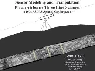
Sensor Modeling and Triangulation for an Airborne Three Line Scanner < 2008 ASPRS Annual Conference >. JAMES S. Bethel Wonjo Jung Geomatics Engineering School of Civil Engineering Purdue University APR-30-2008. Outline. Introduction Dataset Camera Design

E N D
Sensor Modeling and Triangulation for an Airborne Three Line Scanner < 2008 ASPRS Annual Conference > JAMES S. Bethel Wonjo Jung Geomatics Engineering School of Civil Engineering Purdue University APR-30-2008
Outline • Introduction • Dataset • Camera Design • Flight and observations (3-OC Atlanta, GA) • Sensor Model • Trajectory Model • Pseudo Observation Equations • Data Ajustment • Implementation • Results • Conclusions • Future plans
1. Introduction MAIN OBJECTIVE Developing an algorithm to recover orientation parameters for an airborne three line scanner
1. Introduction - Types of three line scanners Three separate cameras Linear arrays on the same focal plane Lens
1. Introduction Instantaneous gimbal rotation center • While ADS40, TLS and JAS placed CCD arrays on the focal plane in a single optical system, 3-DAS-1 and 3-OC use three optical systems, rigidly fixed to each other. • For this reason, we need to develop a photogrammetirc model for three different cameras moving together along a single flight trajectory flight trajectory
1. Introduction • Parameters to be estimated • Exterior orientation parameters • 6 parameters per an image line • Additional external parameters • Translation vector between a gimbal center to perspective centers • Rotation angles between gimbal axis and sensor coordinate systems • Interior orientation parameters • Focal lengths • Principal points • Radial distortions
1. Introduction • There have been two kinds of approaches. • Reducing number of unknown parameters • Piece-wise polynomials • Providing fictitious observations in addition to the real observations • Stochastic models
1. Introduction • Reducing number of unknown parameters • Piecewise polynomials 3×6=18 estimated 1000×6=6000 given
1. Introduction • Providing fictitious observations in addition to the real observations • 1st-Order Gauss-Markov Model observations estimated given
1. Introduction • Self-calibration • Partial camera calibration information is provided. • focal length, aperture ratio, shift of the distortion center, radial distortion • Coordinates of projection center of the camera relative to the gimbal center is not measured. Just design values are provided. • Need to refine some of the parameters
2. DATASET • Camera Design (3-OC)
2. DATASET : 20 GCPs : 8Check points
3. Sensor Model • Collinearity Equation – a line scanner Sensor Coordinate System (SCS) Perspective Center scan line flight direction SCS column row Ground
3. Sensor Model • Collinearity Equation - oblique camera perspective Center scan line flight direction Ground
3. Sensor Model • Collinearity in a three line scanner three angles should be considered flight direction gimbal center B N F plumb line
4. Trajectory Model • 1st order Gauss-Markov trajectory model • Probability density function f(x(t)) at a certain time is dependent only upon previous point • Probability density function is assumed to be Gaussian • Autocorrelation function becomes
4. Trajectory Model • 1st order Gauss-Markov trajectory model autocorrelation function Parameters are highly correlated!
5. Pseudo Observation equations One-sided equation Symmetric pseudo observation equation t autocorrelation function
6. Data Adjustment • the Unified Least Squares Adjustment
7. Implementation • To reduce the number of parameters, only the parameters of lines containing image observations are implemented. • For the memory management, IMSL Ver. 6.0 library is used. IMSL contains a sparse matrix solver. • riptide.ecn.purdue.edu • Red Hat Enterprise Linux 4 operating systems • 16 multi core processors • 64GB of system memory
8. Results • Processing time : 49 seconds (16 core x86_64 Linux with 64GB ram) • Number of iteration : 7 • Converged at 0.58 pixels • RMSE : 1.08 pixels for 8 check points
8. Results • Interior Orientation parameters are self-calibrated
9. Conclusions • We could successfully recover the orientation parameters using stochastic trajectory model • Interior orientation parameters of three cameras can be refined through the self calibration process
9. Future Plans • Analysis on the model properties • Adding pass points • Automated passpoints generation