Download
1 / 60
610 likes | 833 Views
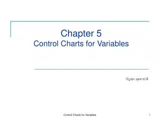
Ch5 Control Charts for Variables. C.C. for process average ( mean quality ):. C.C. for process variability ( dispersion ):. ( 更一般化 ). S chart ; R chart. Variable : numerical measurement A single measurable quality characteristic, such as a

E N D
Ch5 Control Charts for Variables • C.C. for process average(mean quality): • C.C. for process variability(dispersion): (更一般化). S chart;R chart • Variable:numerical measurement • A single measurable quality characteristic, such as a • dimension, weight, or volume, is called a variable.
Process mean及Process variability必須同時control. • (a) Mean and standard deviation at nomial levels.
Process mean is out of control: High fraction of nonconforming product. High process fill out. • Process variability is out of control:
假設quality characteristic is normally distributed with • mean and standard deviation . If is a sample • of sizen, then the average of this sample is Statistical Basis of the Charts 當X 不是Normal,但n 夠大時,上述之C.L.亦可使用。
Center line • 若 與 未知時 其中 每一個都是average of n obs. is called the 從Range估計 Range of (sample of size n) (sample size n 的函數,查 (適用於 ) 其中 relative range. App. VI)
與 的相對效率 n Relative Efficiency 2 3 4 5 6 10 1.000 0.992 0.975 0.955 0.930 0.850 For moderate value of n, say , the range loses efficiency rapidly, as it ignores all the information in the sample between and . 隨n增大而遞減 結論:exhibit in control.
令 C.C. for process mean C.C. for process mean
為n的函數(查 • 中央線 再以 估 C.C. for range 其中 R chart的建法 App. VI)
。Process variability in control 。Process mean in control 結論:Since both and R charts exhibit control, we would conclude that the process is in control at the stated levels and adopt the trial control limits for use in on-line statistical process control. Example 1: 25個samples,每個n=5(見附表) (見附圖) (見附圖)
Specification Process capability的基本定義 Estimating Process Capability 如何評估製造過程的Capability(能力) • 假設活塞環的specification limits是74 ±0.05mm, • 則在上述例子中製造不良活塞環的比率為 • PCR(process capability ratio):另一個評估capability的指標
一般 為未知,以 估計,上述中 或計算 此process的natural tolerance limits佔據 specification band的60% 表示此製造過程的natural tolerance limits是完全落在 USL及LSL之間。
PCR = 1 若在normal假設下,則此process製造出不良品的比率 為0.27%,即2700PPM。 • PCR > 1
PCR < 1 大量的不良品被製造。
Revision of Control Limits and Center Lines (定期的修正C.L.及Center Lines) 例如:每週、每月或每25、50或100個樣本。 • 若R chart顯示in control且process mean僅受單純的variable控制,則可將center line調到target value,但若process mean是被更複雜的variables所控制,則不適宜做此調整。 • 若R chart顯示out of control,則eliminate那些點再重新計算center line和control limit。
活塞環的製造,繼續使用 及R chart. • 如下表及附圖。 • 同時可使用tolerance chart(或稱tier diagram)。 • 當n≧7 or 8時,則可使用Box plot.
CL 、SL及NTL: CL 與SL兩者之間不存在任何數學關係。 • CL是由process的natural variability(即NTL)所決定。 • SP則是由management、engineer、customers…決定 • (即過程外的因素所決定)。 • Control chart使用CL。 • Tolerance chart可用specification limits。
及R chart rational subgroup的選法 1. 對 chart而言 監測process meanbetween sample Sample 1 Sample 2 … Maximize the chance for shifts in 錯誤的估計法!將使S變得太大 且combines了between及within sample的variability. 2. 對R chart而言 監測process variabilitywithin sample 使得variability within samples只測量chance 或random causes
樣本大小 CL的寬度 取樣的頻率 設計C.C.的準則 • CC的統計性質 • 經濟的考量:cost of sampling, costs of investigating • and possibly correcting the process in response to out • of control signals, costs associated with producing a • product that does not meet specifications.
chart若要detect中、大的shift,則n=4、5, • 若要detect小的shift,則n=15、25。 • R chart在n小時,對shift相當insensitive。 • (e.g. n=5,則detect從 到的機率僅有0.4。) • 但n大時(n≧10),則不宜採用R chart,應採用S或 • chart。 • small n 可避免shift發生在一個sample之中。
CL通常取 ,若Type I error甚嚴重,可改採 ,或需 • 在短時間內detect出out of control,則可採用 。 • 取樣頻率:small, frequent or larger samples less frequently, • 目前工業界較偏向於small, frequent的取樣法。 • 取樣頻率可由rate of production決定。
及R chart中n為變數時 • 採用 及S chart(∵R chart的center亦隨時改變)。 • 從某一個時間後開始改變sample size從 。 new
但 與 皆是估計 ,∴若 沒改變
:n↓,CL的寬度↑ :n↓,center line↓及UCL↓ Example 2:活塞環的製造 由於process exhibits good control (見附圖) (見附圖)
Probability Limits on the and R Chart • chart(Normal假設下): • e.g. 2. R chart:由 的percentage points決定。 e.g. If , the 0.001 and 0.999 percentage points of the distribution of the relative range W are required. Noting these points by and 當3≦n≦6,有正的LCL (即由檢定的Type I level所決定的control limit:UK或西歐國家)
In processes where the mean of the quality • characteristic is controlled by adjustments • to the machine, standard or target values of • are sometimes helpful in achieving • management goals with respect to process • performance. • 使用標準值時,需注意out of control的意義!
Interpretation of and R charts • 在解釋 chart上的pattern前,需先檢測R chart是否 • in control?先消去R chart中的assignable causes,再 • 來看 chart. 可能原因: chart:溫度、工作疲乏、 人員或機器輪流、 電壓變動… R chart:maintenance schedules、工作疲乏、工具磨損… e.g.金屬容盤的容量具有systematic的variability,是由於在 filling machine中的compressor開關的週期所造成。 Case 1 Cycles
Case 2 Mixture pattern 可能原因: 是由兩個有overlapping 的分佈來製造此過程的 成品,overlap愈少,此 現象就愈明顯。有時是由於overcontrol所造成。 Case 3 Shift in process level 可能原因: 新進人員、新方法、新 原料、新機器、採用新 的檢測法或標準,改變 skill、目標、或員工的motivations。
可能原因: CL計算錯誤或是 太大,即每次取樣是由數個population 取出,亦即 是測量between population的variability,而不 是within population的variability。 Case 4 Trend 可能原因: tool的持續惡化,operator fatigue、presence of supervisor(或其他的 critical process component)、或分開或合併化學製造過程 中混合物的元素或溫度…(迴歸的控制圖)。 Case 5 Stratification (點不自然的集中在中央 線附近,lack of natural variability!)
The effect of nonnormality on and R charts • 在Normal的假設下, 與R chart互相獨立,若否,則 • 表示Normality的假設不適合,即分佈可能是skewed! • 當品質的特性的underlying分佈可由過去收集的大量資 • 料來統計,則可藉此計算其probability limit,進而建立 • CC,但在大部份的情況,underlying的分佈是不可知, • 則我們想了解CC對normality假設的robustness性質。
E.g. chart:uniform、 right triangular、 gamma( )n=4,5時 robustness 最差的情況:gamma(r=1/2,1(exponential)) (gamma ) R chart:即使當分佈是normal,R的分佈亦非對稱, 一般使用的 3-sigma limit,其 (當n=4),且R chart較 chart對normality的假設更 sensitive!
In control value 當 已知時, chart的O.C. curve 當 的 The Operating-Characteristic Function (如附圖) (在第k個sample(after the shift)才detect出shift的機率) (此即為幾何分佈的期望值)
In control value of the standard deviation 其中 ,查 的表 R chart的O.C. curve (如附圖) 利用O.C. curve來分析過去的資料,建議一般取20~25 subgroups來建立C.C. 。
The Average Run Length for the Chart 皆為幾何分佈的期望值 (如附圖) Average Time to Signal:ATS=ARL.k Expected number of individual units sampled: I=nARL (如附圖)
1. The sample size n is moderately large, say n>10 or 12. (Recall that the range method for estimating loses statistical efficiency for moderate to large samples.) Control charts for and S 使用 及S charts。 當 2. The sample size n is variable.
是 的unbiased estimator Construction and Operation of and S Charts S並非 的不偏估計量,但 , 其中
當standard value is given S chart 當 是未知,則以 ,估計 S chart
chart 注意: 若取 , 則相對的 均隨著改變, 並改以 的符號來代表。
Example 3 活塞環的內半徑(如下表)
與先前的 相似(如下圖) 與由 估計的值相近
The and S Control Charts with Variable Sample Size chart 當n是個變數時 其中 將由individual subgroup來決定 S chart
Example 4 活塞環內半徑n=3~n=5(如下表)
chart S chart 對第二個sample,n=3時, 的值亦隨之改變。 對第一個sample,n=5的C.L. (如附表與附圖)
當n是變數時,另一個可行的方法是採用 • average sample size • (適用於 變化不大時或展示給 manager看時) • 亦利用最常出現的 值來估計 的值。 • e.g.在Example 4中, 共有17 個,為最常出現的 • 值,則 • used is for samples of size n=5.
The Control Chart (recommended by some practitioners)
若無法給定standards,通常以20~25preliminary samples • 的資料來建立trial control limits,但m=20~25對某些過 • 程而言卻太大(如start up process)。若m(即sample數) • 取得太小,則造成 變大。 e.g. chart中, 即使當m=25時,亦比nominal value大。 解決方法為:Hillier(1969)Two stage approach 來建立C.L. for and R charts.使得不論m之值為何, 皆可有正確的 值可應用於 job-shop or short production run。 Control Limits Base on a Small Number of Samples (Short Production Runs)
Control Charts for Individual Measurements • 當n=1的例子 • 1. 自動化偵測每個產品。 • 2. 生產速度甚慢,不便取n>1。 • 3. 重覆測量的差異僅是由實驗或分析的錯誤所產生, • (e.g. 化學過程),即重覆測量是不需要的。 • 4. 例如在一捲紙中塗料的厚度,幾乎是處處相同, • 重覆取樣是不需要的,其所得的std. dev.亦會太小。
可利用相鄰觀測值的moving range來估計process的 • variability,即 • 當要detect的shift很小時,則可採用Ch 7的cumulative • sum及exponential weighted moving-average C.C. 。
Example 5 • 飛機底漆的黏性是 • 一個重要的品質。 • 數個小時才能生產 • 一個batch的油漆, • 因此每次取樣僅能 • 取一個batch。