Lecture 6. Prefix Complexity K
Lecture 6. Prefix Complexity K. The plain Kolmogorov complexity C(x) has a lot of “minor” but bothersome problems

Lecture 6. Prefix Complexity K
E N D
Presentation Transcript
Lecture 6. Prefix Complexity K • The plain Kolmogorov complexity C(x) has a lot of “minor” but bothersome problems • Not subadditive: C(x,y)≤C(x)+C(y) only modulo a logn factor. There exists x,y s.t. C(x,y)>C(x)+C(y)+logn –c. (This is because there are (n+1)2n pairs of x,y s.t. |x|+|y|=n. Some pair in this set has complexity n+logn. • Nonmonotonicity over prefixes • Problems when defining random infinite sequences in connection with Martin-Lof theory where we wish to identify infinite random sequences with those whose finite initial segments are all incompressible, Lecture 2 • Problem with Solomonoff’s initial university distribution P(x) = 2-C(x) but P(x)=∞.
In order to fix the problems … • Let x=x0x1 … xn , then x =x00x10x20 … xn1 and x’=|x| x • Thus, x’ is a prefix code such that |x’| ≤ |x|+2 log|x| • x’ is a self-delimiting version of x. • Let reference TM’s have only binary alphabet {0,1}, no blank B. The programs p should from an effective prefix code: p,p’ [ p is not prefix of p’] • Resulting self-delimiting Kolmogorov complexity (Levin, 1974, Chaitin 1975). We use K for prefix Kolmogorov complexity to distinguish from C, the plain Kolmogorov complexity.
Properties • By Kraft’s inequality (proof – look at the binary tree): x * 2-K(x) ≤ 1 • Naturally subadditive • Monotonic over prefixes • C(x) ≤ K(x) ≤ C(x)+log C(x) • K(x|n) ≤ K(x) + O(1) ≤ C(x|n) + K(n)+O(1) ≤ C(x|n)+log*n+logn+loglogn+…+O(1) • An infinite binary sequence ω is (Martin-Lof) random iff there is a constant c s.t. for all n, K(ω1:n)≥n-c. (Note, please compare with Lecture 2, C-measure)
Alice’s revenge • Remember Bob at a cheating casino flipped 100 heads in a row. • Now Alice can have a winning strategy. She proposes the following: • She pays $1 to Bob. • She receives 2100-K(x) in return, for flip sequence x of length 100. • Note that this is a fair proposal as |x|=100 2-100 2100-K(x) < $1 But if Bob cheats with 1100, then Alice gets 2100-log100
Chaitin’s mystery number Ω Define Ω = ∑P halts on ε2-|P| <1 by Kraft’s inequality. Theorem 1. Let Xi=1 iff the ith program halts. Then Ω1:n encodes X1:2^n. I.e., from Ω1:n we can compute X1:2^n Proof. (1) Ω1:n < Ω < Ω1:n+2-n. (2) Dovetailing simulate all programs till Ω’> Ω1:n. Then if P, |P|≤n, has not halted yet, it will not (since otherwise Ω > Ω’+2-n> Ω). QED • Bennett: Ω1:10,000 yields all interesting mathematics. Theorem 2. K(Ω1:n) ≥n – c. • Remark. Ω is a particular random sequence! Proof. By Theorem 1, given Ω1:n we can obtain all halting programs of length ≤ n. For any x that is not an output of these programs, we have K(x)>n. Since from Ω1:n we can obtain such x, it must be the case that K(Ω1:n) ≥n – c. QED
Universal distribution • A (discrete) semi-measure is a function P that satisfies xNP(x)≤1. • A enumerable semi-measure P0 is universal (maximal) if P0 if for all enumerable semi-measure P, there is a constant cp, s.t. for all xN, cPP0(x)≥P(x). We say that P0 dominates each P. Theorem. There is a universal enumerable semi-measure, m. Theorem. –log m(x) = K(x) + O(1) ---- Proof omitted. • Remark. This universal distribution m is one of the foremost notions in KC theory. As prior probability in a Bayes rule, it maximizes ignorance by assigning maximal probability to all objects (as it dominates other distributions up to a multiplicative constant).
Average-case complexity under m Theorem [Li-Vitanyi]. If the input to an algorithm A is distributed according to m, then the average-case time complexity of A equals to A’s worst-case time complexity. Proof. Let T(n) be the worst-case time complexity. Define P(x) as follows: • an=|x|=nm(x) • If |x|=n, and x is the first s.t. t(x)=T(n), then P(x):=an else P(x):=0. Thus, P(x) is enumerable, hence cPm(x)≥P(x). Then the average time complexity of A under m(x) is: T(n|m) = |x|=nm(x)t(x) / |x|=nm(x) ≥ 1/cP |x|=n P(x)T(n) / |x|=nm(x) = 1/cP |x|=n [P(x)/|x|=nP(x)] T(n) = 1/cPT(n). QED Intuition: The x with worst time has low KC, hence large m(x) Example: Quicksort. With easy inputs, more likely incur worst case.
Inductive Inference • Solomonoff (1960, 1964): given a sequence of observations: S=010011100010101110 .. • Question: predict next bit of S. • Using Bayesian rule: P(S1|S)=P(S1)P(S|S1) / P(S) =P(S1) / [P(S0)+P(S1)] here P(S1) is the prior probability, and we know P(S|S1)=P(S|S1)=1. • Choose universal prior probability: P(S) = 2-K(S) , denoted as m(x) • Continue in Lecture 7 on this topic.