UNIT-2 Multiple Random Variable
Understand vector random variables, joint probability, independence, and conditional probability. Learn how to model systems and calculate probabilities using vector random variables. Explore examples and applications.

UNIT-2 Multiple Random Variable
E N D
Presentation Transcript
UNIT-2 Multiple Random Variable • 4.1 Vector Random Variables • 4.2 Pairs of Random Variables • 4.3 Independence of Two Random Variables • 4.4 Conditional Probability and Conditional Expectation • 4.5 Multiple Random Variables • 4.6 Functions of Several Random Variables • 4.7 Expected Value of Functions of Random Variables • 4.8 Jointly Gaussian Random Variables
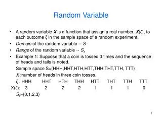
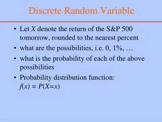
2.1 Vector Random Variables A vector random variableX is a function that assigns a vector of real numbers to each outcome ζ in S, the sample space of the random experiment . EXAMPLE 4.1 Let a random experiment consist of selecting a student’s name form an urn. Let ζdenote the outcome of this experiment, and define the following three functions :
Events and Probabilities EXAMPLE 2.4 Consider the tow-dimensional random variable X = (X, Y). Find the region of the plane corresponding to the events The regions corresponding to events A and C are straightforward to find and are shown in Fig. 4.1.
For the n-dimensional random variable X = (X1,…,Xn), we are particularly interested in events that have the product form where Ak is a one-dimensional event (ie., subset of the real line) that involves Xk only. A fundamental problem in modeling a system with a vector random variable X = (X1,…, Xn) involves specifying the probability of product-form events : In principle, the probability in Eq. (4.2) is obtained by finding the probability of the equivalent event in the underlying sample space,
EXAMPLE 4.5 None of the events in Example 4.4 are of product form. Event B is the union of two product-form events :
The probability of a non-product-form event B is found as follow : First, B is approximated by the union of disjoint product-form events, say, B1, B2,…, Bn; the probability of B is then approximated by The approximation becomes exact in the limit as the Bk’s become arbitrarily fine. Independence If the one-dimensional random variable X and Y are “independent,” if A1 is any event that involves X only and A2 is any event that involves Y only, then
In the general case of n random variables, we say that the random variables X1, X2,…, Xn are independent if where the Ak is an event that involves Xk only.
2.2 PAIRS OF RANDOM VARIABLES Pairs of Discrete Random Variable Let the vector random variable X = (X,Y) assume values from some countable set The joint probability mass function of X specifies the probabilities of the product-form event The probability of any event A is the sum of the pmf over the outcomes in A :
The fact that the probability of the sample space S is 1 gives The marginal probability mass functions : and similarly,
EXAMPLE 2.7 The number of bytes N in a message has a geometric distribution with parameter 1-p and range SN={0, 1, 2, …}. Suppose that messages are broken into packets of maximum length M bytes . Let Q be the number of full packets in a message and let R be the number of bytes left over. Find the joint pmf and the marginal pmf’s of Q and R. SQ={0, 1, 2,….} and SR={0, 1, 2, ….M – 1} . The probability of the elementary event {(q, r)} is given by The marginal pmf of Q is
The Joint cdf of X and Y The joint cumulative distribution function of X and Y is defined as the probability of the product-form event The joint cdf is nondecreasing in the “northeast” direction, It is impossible for either X or Y to assume a value less than , therefore It is certain that X and Y will assume values less than infinity, therefore
If we let one of the variables approach infinity while keeping the other fixed, we obtain the marginal cumulative distribution functions and Recall that the cdf for a single random variable is continuous form the right. It can be shown that the joint cdf is continuous from the “north” and from the “east” and
EXAMPLE 2.8 The joint cdf for the vector of random variable X = (X,Y) is given by Find the marginal cdf’s. The marginal cdf’s are obtained by letting one of the variables approach infinity :
The cdf can be used to find the probability of events that can be expressed as the union and intersection of semi-infinite rectangles. Consider the strip defined by denoted by the region B in Fig. 4.6(a) . By the third axiom of probability we have that The probability of the semi-infinite strip is therefore Consider next the rectangle denoted by the region A in Fig 4.6 (b).
The probability of the rectangle is thus EXAMPLE 2.9 Find the probability of the events where x > 0 and y > 0, and in Example 4.8 The probability of A is given directly by the cdf : The probability of B requires more work. Consider Bc
The probability of the union of two events : The probability of B : The probability of event D is found by applying property vi of the joint cdf :
The Joint pdf of Two Jointly Continuous Random Variables We say that the random variables X and Y are jointly continuous if the probabilities of events involving (X, Y) can be expressed as an integral of a pdf. There is a nonnegative function fX,Y(x,y), called the joint probability density function, that is defined on the real plane such that for every event A, a subset of the plane, as shown in Fig. 4.7. When a is the entire plane, the integral must equal one : The joint cdf can be obtained in terms of the joint pdf of jointly continuous random variables by integrating over the semi-infinite
rectangle defined by (x, y) : It then follows that if X and Y are jointly continuous random variables, then the pdf can be obtained from the cdf by differentiation : The probability of a rectangle region is obtained by letting in Eq. (4.9) :
The marginal pdf’s fX(x) and fY(y) are obtained by taking the derivative of the corresponding marginal cdf’s , and Similarly,
EXAMPLE 2.10 Jointly Uniform Random Variables A randomly selected point (X, Y) in the unit square has the uniform joint pdf given by Find the joint cdf. There are five cases in this problem, corresponding to the five regions shown in Fig. 4.9. 1. If x < 0 or y < 0, the pdf is zero and Eq. (4.12) implies 2. If (x,y) is inside the unit interval,
3. If 4. Similarly, if 5. Finally, if
EXAMPLE 2.11 Find the normalization constant c and the marginal pdf’s for the following joint pdf : The constant c is found from the normalization condition specified by Eq. (4.10) : Therefore c= 2. The marginal pdf’s are found by evaluating Eq. (4.15a) and (4.15b) : and
EXAMPLE 2.13 Jointly Gaussian Random Variables The joint pdf of X and Y, shown in Fig. 4.11 is We say that X and Y are jointly Gaussian. Find the marginal pdf’s. The marginal pdf of X is found by integrating fX,Y(x,y) over y : We complete the square of the argument of the exponent by adding and subtracting ρ2x2 , that is
Random Variables That Differ in Type EXAMPLE 2.14 A Communication Channel with Discrete Input and continuous Output Let X be the input , Y be output and N be noise. and Find therefore where P[X = +1] = 1 / 2. When the input X = 1, the output Y is uniformly distributed in the interval [-1, 3]; therefore
2.3 INDEPENDENCE OF TWO RANDOM VARIABLES X and Y are independent random variables if any event A1 defined in terms of X is independent of any event A2 defined in terms of Y ; Suppose that X and Y are a pair of discrete random variables. If we let then the independence of X and Y implies that Therefore, if X and Y are independent discrete random variables, then the joint pmf is equal to the product of the marginal pmf’s
Let be a product-form event as above, then We say, The “discrete random variables X and Y are independent if and only if the joint pmf is equal to the product of the marginal pmf’s for all xj, yk ”
EXAMPLE 4.16 Are Q and R in Example 4.7 independent? From Example 4.7 we have Therefore Q and R are independent.
It can shown that the random variables X and Y are independent if and only if their joint cdf is equal to the product of its marginal cdf’s : Similarly, if X and Y are jointly continuous, then X and Y are independent if and only if their joint pdf is equal to the product of the marginal pdf’s : EXAMPLE 4.18 Are the random variables X and Y in Example 4.13 independent? The product of the marginal pdf’s of X and Y in Example 4.13 is The jointly Gaussian r.v’s X and Y are indepdent if and only if ρ=0.
EXAMPLE 4.19 Are the random variables X and Y independent in Example 4.8? If we multiple the marginal cdf’s found in Example 4.8 we find so X and Y are independent. If X and Y are independent random variables, then the random variables defined by any air of functions g(X) and h(Y) are also independent. 1. Consider the one-dimensional events A and B. 2. Let A’ be the set of all values of x such that if x is in A’ then g(x) is in A,
2.4 CONDITIONAL PROBABILITY AND CONDITIONAL EXPECTATION Conditional Probability In Section 2.4, we know If X is discrete, then Eq. (4.22) can be used to obtain the conditional cdf of Y given X = xk: The conditional pdf of Y given X = xk , if the derivative exists, is given by
Integrating the conditional pdf : Note that if X and Y are independent, so If X and Y are discrete, then for xk such that . We defined for xk such that . The probability of any event A given X = xk is found by
Note that if X and Y are independent, then EXAMPLE 4.20 Let X be the input and Y the output of the communication channel discussed in Example 4.14. Find the probability that Y is negative given that X is +1. If X =+1, then Y is uniformly distributed in the interval [-1, 3], that is ,
Thus If X is a continuous random variable, then P[X = x] = 0 so Eq. (4.22) is undefined. We define the conditional cdf of Y given X = x by the following limiting procedure: The conditional cdf on the right side of Eq. (4.28) is :
As we let h approach zero, The conditional pdf of Y given X = x is obtained by Note that if X and Y are independent, then
EXAMPLE 2.21 Let X and Y be the random variables introduced in Example 4.11. Find Using the marginal pdf’s and
If we multiply Eq. (4.26) by P[ X = xk], then Suppose we are interested in the probability that Y is in A :
If X and Y are continuous, we multiply Eq. (4.31) by fX(x) To replace summations with integrals and pmf’s with pdf’s , EXAMPLE 2.22 Number of Defects in a Region; Random Splitting of Poisson Counts The total number of defects X on a chip is a Poisson random variable with mean α. Suppose that each defect has a probability p of falling in a specific region R and that the location of each defect is independent of the locations of all other defects. Find the pmf of the number of defects Y that fall in the region R. Form Eq. (4.33)
The total number of defect : X = k, the number of defects that fall in the region R is a binomial r.v with k, p Noting that Thus Y is a Poisson r.v with mean αp.
EXAMPLE 2.23 Number of Arrivals During a Customer’s Service Time The number of customers that arrive at a service station during a time t is a Poisson random variable with parameter βt. The time required to service each customer is an exponential random variable with parameter α. Find the pmf for the number of customers N that arrive during the service time T of a specific customer. Assume that the customer arrivals are independent of the customer service time.
Let r = (α+β)t, then where we have used the fact that the last integral is a gamma function and is equal to k!. Conditional Expectation The conditional expectation of Y given X = x is defined by If X and Y are both discrete random variables, we have