Download
1 / 28
280 likes | 316 Views
Learn how to eliminate redundant states in sequential networks through state reduction techniques. Understand how equivalent states are identified and removed to optimize network efficiency.

E N D
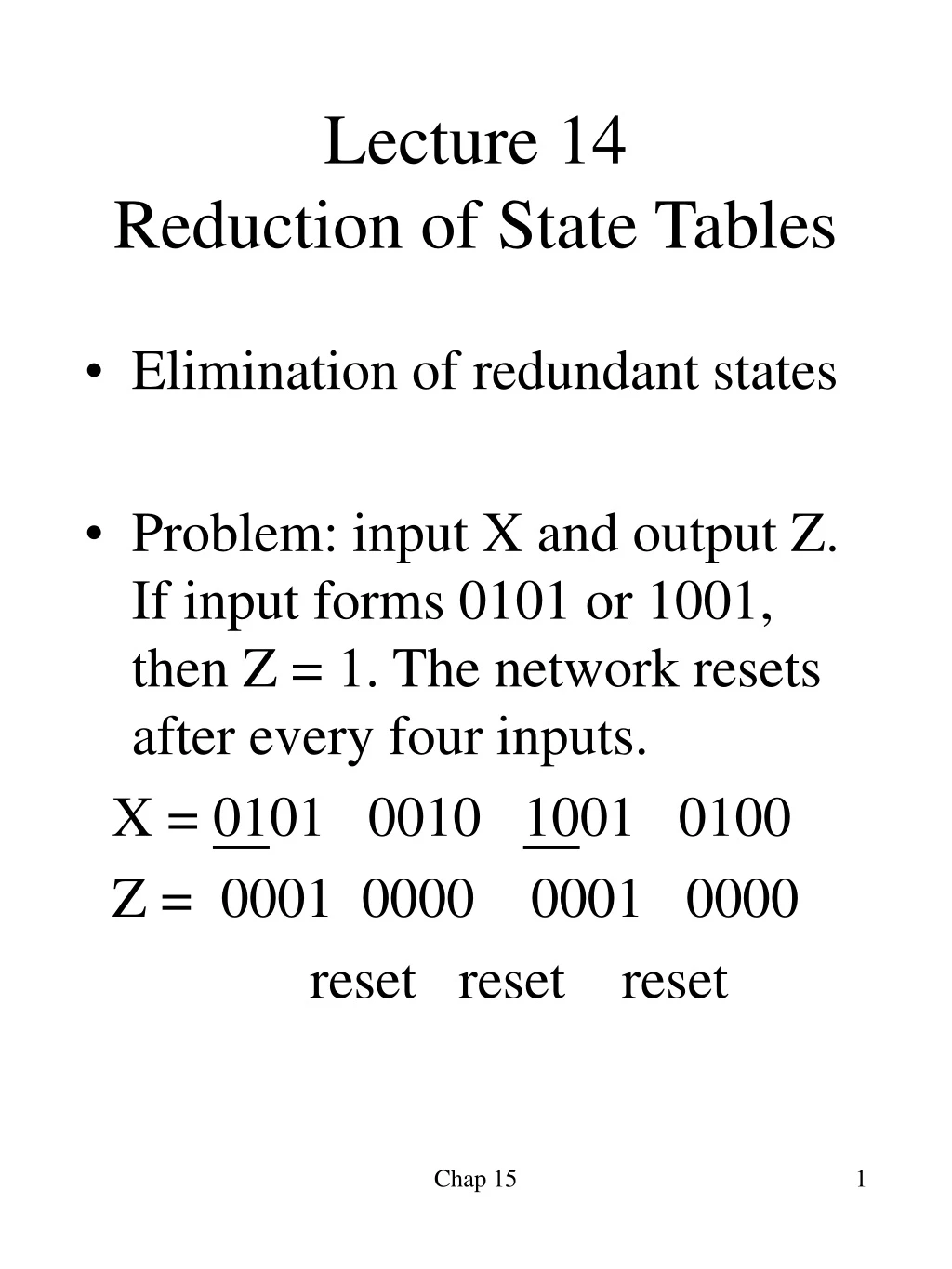
Lecture 14 Reduction of State Tables • Elimination of redundant states • Problem: input X and output Z. If input forms 0101 or 1001, then Z = 1. The network resets after every four inputs. X = 0101 0010 1001 0100 Z = 0001 0000 0001 0000 reset reset reset Chap 15
Elimination of redundant states • Designate each next state as a bit is received. We may have redundant states. 0101 or 1001 Chap 15
Elimination of redundant states • Find the equivalent states and eliminate those that have the same next state and outputs. • (I, K, M, N, P => H, keep H) Chap 15
Elimination of redundant states (cont.) • Row matching: sufficient only to network reset to the starting state after receiving a fixed number of inputs. Chap 15
Equivalent States ≡ • Equivalent: two states are equivalent if there is no way of telling them apart from observation of network inputs and outputs. • N1: started in state p • N2: started in state q. • For every possible input sequence X, the output sequences are the same (Z1 and Z2). Then we say that p is equivalent to q. Chap 15
Equivalent States • State p in N1. • State q in N2. • Output sequence is a function of the initial state and input sequence. Then, • We have Z1 = λ1(p,X) and Z2= λ2 (q, X). • State p in N1 is equivalent to state q in N2 iff Z1 = Z2 for every possible input sequence X. • X = X1, X2, X3 …. • Z1 = Z1, Z2, Z3….. Chap 15
Theorem • Two states p and q of a sequential network are equivalent iff for every single input X, the outputs are the same and the next states are equivalent, that is, • λ(p,X) = λ(q,X) (output) and • δ(p, X) ≡ δ(q, X) (next state) Where λ(p,X) is the output given the present state p and input X and δ(p, X) is the next state given the present state p and input X. Chap 15
Application of the Theorem • Are S0 and S2 equivalent? • Present output is the same for S0 and S2. • S0 ≡ S2 iff S3 ≡ S3, S2 ≡ S0, S1 ≡ S1 and S0 ≡ S1. But S0 ≡ S1 (due to outputs.) • The answer is No. Chap 15
Implication Table for State Equivalence • Use an implication table (pair chart) to check each pair of states for possible equivalence. Chap 15
Implication Table for State Equivalence (cont.) • a ≡ b iff d ≡ f and c ≡ h. This “implied pair” is placed in a-b square. Self-implied pairs are redundant. So eliminate them. a ≡ d iff a ≡ d and c ≡ e. Chap 15
Implication Table for State Equivalence (cont.) • For a-b square, we need d≡f and c≡h for a≡b. But in the d-f square we see a X which means that d is not equivalent to f. So a is not equivalent to b. We place a X in the a-b square. • For a-d square, square c-e does not contain a X. So at this point, we can not determine whether a ≡d. • Do the first pass column by column. Chap 15
Implication Table for State Equivalence (cont.) • After the first pass, we do the second pass from a column again. Then, we do the third pass and find no new X’s are added. Then the process terminates. • The result is a ≡d and c ≡e. • So we replace d with a and e with c and eliminate row d and e. Chap 15
Equivalent Sequential Networks • Sequential network N1 is equivalent to sequential network N2 if for each state p in N1 there is a state q in N2 such that p q, and conversely, for each state s in N2 there is a state t in N1 such that s t. • That is, for N1 and N2, the output sequences are the same for the same input sequences. Chap 15
Equivalent Sequential Networks (cont.) • A S2? (output is the same). IF A S2, then B S0. This further implies D S1 and C S3. This is true from the table. (Next states are equivalent and outputs are the same.) Chap 15
Equivalent Sequential Networks (cont.) • Using implication table to determine network equivalence, place X in the square for different outputs for the compared pair. A S2, B S0, etc Chap 15
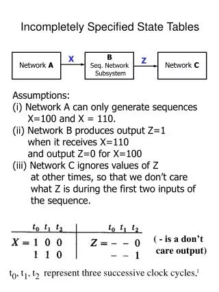
Incompletely Specified State Table • Problem statement • X only has X = 100 and X = 110 sequence • Z for X = 100 is 0. • Z for X = 110 is 1. • Come up each possible state. Chap 15
Incompletely Specified State Table(cont.) • Unspecified states or outputs. • For the next state of S0, X = 0 does not occur. (S0 : reset) • Entering t1, we have S2 or S3 two states depending on X. • Fill in don’t cares for row matching. Chap 15
Derivation of Flip-Flop Input Equations • 3 FFs for 7 states Chap 15
Equivalent State Assignment • State assignment for 3 states S0, S1, and S2. (Table 14-, 101 detector) • We need 2 FFs. S0 can have 00, 01, 10, or 11. In this way, there are 4x3x2x1 = 24 possible combinations to evaluate. • Assignment 1 and assignment 3 has the same cost. Since only the labeling of FF is changed. (change column = same cost) • Assignment 4 and 6 has row change. They will have different cost. Different cost AB Chap 15 Same cost
Interchanging or Complementing State Assignment • Assignment b: interchanging the column of a • Assignment c: complementing the columns of a. • For J-K FF, the cost is the same for all three assignments for any kind of logic gates. • For D FF, if AND and OR gates are available, then the cost is the same. Chap 15
Minimum Cost Realization of State Assignment • Nonequivalent assignment: by eliminating states that can be obtained by permuting or complementing columns. • We can complement one or more columns. So any state assignment can be converted to one in which the first state is assigned all 0’s. • For symmetrical FFs, need only to try three assignments for minimum cost. • The number of distinct states increasesrapidly as the number of states increases. Chap 15
Guidelines for State Assignment • Try to places 1’s on the FF input maps in adjacent squares. • 1: States which have the same next state for a given input should be given adjacent assignment. • 2: States which are the next states of the same state should be given adjacent assignment. • 3: States which have the same output for a given input should be given adjacent assignment (for output simplification.) Chap 15
Guidelines for State Assignment: Example • G1: (S0, S1,S3, S5) (S3, S5) (S4,S6) (S0,S2,S4,S6) S1 as the next state. • G2: (S1, S2) (S2, S3) (S1,S4) (S2,S5)2x (S1,S6)2x • Try to fulfill as many of these adjacency conditions as possible. • G1 preference > G2 preference. Chap 15
Why is it a better assignment? • Next state map shows that S1 appears in four adjacent squares, and etc. Example: S1 = 110 S5 =101 S1 = 110 Chap 15
On State Assignment • In some cases, the assignment which satisfies the most guidelines is not necessarily the best assignment. Therefore, it is a good idea to try several assignments which satisfy most of the guidelines and choose the one which gives the lowest cost function. • In general, the best assignment for one type of flip-flop is not the best for another type. Chap 15
State Assignment for CPLDs • In CPLDs, FPGAs, a logic cell has one or more FFs. • FFs are there whether used or not. • May not be important to minimize the # of FFs used in the design. • Need to reduce the logic cells used and the interconnection between cells for shorter delay. LCs are cascaded to realize a function. So min # of LCs !! • In order design fast logic, minimize the # of cells used. Delay FF0 to FFi FF0 to FFi A logic cell cascaded Chap 15
One-Hot State Assignment • Use one FF for each state. • For a 4-state machine, use 4 FFs. • S0 =Q0Q1Q2Q3 = 1000, S1 :0100, S2: 0010, S3:0001. • Q3+ = X1(Q0Q1’Q2’Q3’) + X2(Q0’Q1Q2’Q3’) + X3(Q0’Q1’Q2Q3’) + X4(Q0’Q1’Q2’Q3) : this is AND • Q3+ = X1Q0 + X2Q1 + X3Q2 + X4Q3 reduced Q+ • Each term contains only one state variable (fewer variables). • More next-state equations are required (FFs are there.) • One FF is reset to 1 instead of resetting all FFs to 0 when resetting the system. • But next state and output equations may contain fewer variables, meaning that fewer logic cells are required. Z2 = X2Q1 + X4 Q3 Chap 15
IN CPLD and FPGA • Try both for state assignment • Minimum number of states • One-hot assignment • And see which leads to the use of the smallest number of logic cells. • Less delays, higher speed! Chap 15