Download
1 / 54
540 likes | 620 Views
Dive into the spatial distribution and dark matter haloes hosting galaxies to understand galaxy formation in the high redshift Universe. Discover how galaxies trace dark matter structure on large scales using emission lines as tracers.

E N D
Lyα emitters in galaxy formation models Alvaro Orsi Cedric Lacey Carlton Baugh Supercomputing techniques in Astrophysics workshop
Emission-line Galaxies • Galaxies with detectable emission lines • Tracers of star formation activity • UV →Lyα,Hα, Hβ, [OII], [OIII],...
Motivation • Spatial distribution • Infer mass of dark matter haloes hosting galaxies • Galaxy formation in the high redshift Universe • What ingredients do we need? • Dark energy surveys - How galaxies trace DM structure on very large scales?
Motivation Orsi et al (2009) • Spatial distribution • Infer mass of dark matter haloes hosting galaxies • Galaxy formation in the high redshift Universe • What ingredients do we need? • Dark energy surveys - How galaxies trace DM structure on very large scales? Emission line galaxies at z=1
Motivation Orsi et al (2009) • Spatial distribution • Infer mass of dark matter haloes hosting galaxies • Galaxy formation in the high redshift Universe • What ingredients do we need? • Dark energy surveys - How galaxies trace DM structure on very large scales? H-band selected galaxies at z=1
Motivation Orsi et al (2009) • Spatial distribution • Infer mass of dark matter haloes hosting galaxies • Galaxy formation in the high redshift Universe • What ingredients do we need? • Dark energy surveys - How galaxies trace DM structure on very large scales? Luminosity function of Hα emitters at z ~ 1
Motivation • Spatial distribution • Infer mass of dark matter haloes hosting galaxies • Galaxy formation in the high redshift Universe • What ingredients do we need? • Dark energy surveys - How galaxies trace DM structure on very large scales? Euclid space mission: Hα emitters slitless survey, 0.5<z<2
Motivation • Spatial distribution • Infer mass of dark matter haloes hosting galaxies • Galaxy formation in the high redshift Universe • What ingredients do we need? • Dark energy surveys - How galaxies trace DM structure on very large scales? HETDEX: Lyα emitters IFU survey at 3<z<5
Lyα emitters Narrow band Lyα search • Hydrogen recombination line • Strongest transition • λ0 = 1216 Å • Tracer of high redshift galaxies (2 < z < 7), aiming to z > 7 • Resonant scattering + dust Small fraction of photons escape from the galaxy Lyα spectrum at z=3 (Gronwall et al. 2006)
Modelling Lyα emitters • We use the semi-analytic model GALFORM developed at Durham • Simulate galaxy populations in cosmological volumes • Star formation and galaxy merger history from first principles
Modelling Lyα emitters • Lyα emitters are modelled using the Baugh et al (2005) model: - Kennicut IMF for quiescent galaxies • Top-heavy IMF for starbursts • SN + Superwind mode of feedback • Monte Carlo merger trees • Lyα emitters have a fixed escape fraction • fesc(Lyα) = 0.02 • constant!
Motivation for Baugh model • Baugh et al (2005) model was not designed to predict Lyα emitters properties : • Submillimitre number counts and redshift distributions • Luminosity function of Lyman break galaxies • Galaxy evolution in the IR (Lacey et al 2008, 2009) Baugh et al (2005)
Motivation for Baugh model Baugh et al (2005) • Baugh et al (2005) model was not designed to predict Lyα emitters properties : • Submillimitre number counts and redshift distributions • Luminosity function of Lyman break galaxies • Galaxy evolution in the IR (Lacey et al 2008, 2009)
Evolution of Lyα LF Orsi et al (2008) Luminosity functions well reproduced in a wide range of redshifts, even with a fixed escape fraction!
Evolution of Lyα LF Orsi et al (2008) Luminosity functions well reproduced in a wide range of redshifts, even with a fixed escape fraction!
Evolution of Lyα LF Orsi et al (2008) Luminosity functions well reproduced in a wide range of redshifts, even with a fixed escape fraction!
Spatial distribution • We combine GALFORM with the Millennium Simulation • Box size: 500[Mpc/h] • Mhalo > 1.72 x 10¹⁰ M/h • Alternatively, N-body merger trees can be used
Lyα emitters at z = 0 • Low abundance due to modest star formation activity Dark matter Galaxies
Lyα emitters at z = 3.3 • Near peak of star • formation activity
Lyα emitters at z = 5.7 • Star formation • decreases again
Lyα emitters at z = 8.5 • Star formation • decreases more
Clustering of Lyα emitters Two point correlation function fit by:
Comparing to observational data Mock catalogues of SXDS • Median w() of mock catalogues
Comparing to observational data Mock catalogues of SXDS • Median w() of mock catalogues • Idealized survey over much larger solid angle
Comparing to observational data Mock catalogues of SXDS • Median w() of mock catalogues • Idealized survey over much larger solid angle • Model agrees with observational measurements at 95% confidence
Comparing to observational data Mock catalogues for MUSYC, z=3 Abundances and clustering properties are well reproduced in a constant escape fraction scenario!
But, is the escape fraction constant? Atek et al (2009)
Empirical attempts to model fesc Kobayashi et al (2008, 2009) semianalytic model
Empirical attempts to model fesc Nagamine et al. (2008) SPH simulation Escape fraction scenario: Duty cycle scenario Samples diluted by a fixed fraction
Empirical attempts to model fesc Nagamine et al. (2008) SPH simulation Escape fraction scenario: Duty cycle scenario Samples diluted by a fixed fraction
Detailed modelling of Lyα photons • Monte Carlo Radiative Transfer • Follow scattering of Lyα photons by HI atoms in the ISM • How many of them escape (effect of dust) • Lyα spectrum • Some applications: • Understand observed line profiles • Verhamme et al. (2006,2008), • Surface brightness of Lyα emission in • SPH galaxies • Laursen et al (2008,2009) • Modelling observed DLAs • Dijkstra et al (2006), Barnes et al (2009) • Neutral gas fracion in the IGM • - Cantalupo et al (2008)
The Monte Carlo code • Define the properties of the HI region (geometry, density, temperature, kinematics, etc) The frequency of the photon is characterised by
The Monte Carlo code 2. Choose the location and direction and frequency of the photon 3. The photon will travel an optical depth given by
The Monte Carlo code 4. At the location of interaction, we calculate the probability of interacting with an H atom 5.1 If the photon interacts with dust, then the dust albedo A tells us whether the photon was absorbed or scattered. If absorbed, then the photon is lost and we start over again.
The Monte Carlo code 5.2 If interacts with hydrogen then we compute the cross section: The velocity of the atom parallel to the direction of the photon depends on its frequency:
The Monte Carlo code 6. We perform a Lorentz transformation to the atom’s frame to compute the frequency and direction after the scattering 7. We repeat the process until the photon escapes or is absorbed. The same is applied to a large number of photons
Lyα spectrum Homogeneous, static slab Harrington (1973) analytical prediction τ0=104
Lyα spectrum Homogeneous, static slab Harrington (1973) analytical prediction τ0=104 τ0=105
Lyα spectrum Homogeneous, static slab Harrington (1973) analytical prediction τ0=104 τ0=105 τ0=106
Lyα spectrum Homogeneous, static sphere Dijkstra (2006) analytical prediction
Escape fraction for homogeneous slab Analytical solution for this case (Neufeld, 1990) No analytical solution for more general cases
Effect of outflow velocity Homogeneous expanding sphere Static case
Effect of outflow velocity Homogeneous expanding sphere Vmax=20 km/s: Photons are slightly redshifted
Effect of outflow velocity Homogeneous expanding sphere Vmax=200 km/s: Photons are completely redshifted
Effect of outflow velocity Homogeneous expanding sphere Vmax=2000 km/s: The optical depth becomes so thin that photons escape very easily after being redshifted
Next step • Combine with GALFORM • Choose a suitable geometry for the ISM • Study dependence of escape fraction on mass, redshift, luminosities, metallicities, etc...
Measuring BAOs with Hα emitters Orsi et al (2009)
Tracing large scale structure with Hα emitters • Forthcoming dark energy space missions will measure BAOs using Hα emitters • To what accuracy? Understand Hα emitters from a galaxy formation perspective