Geometry and Fields:

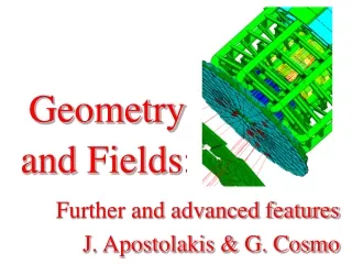
1. Geometry and Fields: Further and advanced features J. Apostolakis & G. Cosmo

2. PART I Detector DescriptionAdvanced features Debugging tools Creating geometry in simpler way The Geant4 Geometrical Editor (tabular) Grouping volumes Reflections of volumes and hierarchies User defined solids Interface to CAD systems

3. Debugging geometries • An overlapping volume is a contained volume which actually protrudes from its mother volume • Volumes are also often positioned in a same volume with the intent of not provoking intersections between themselves. When volumes in a common mother actually intersect themselves are defined as overlapping • Geant4 does not allow for malformed geometries • The problem of detecting overlaps between volumes is bounded by the complexity of the solid models description • Utilities are provided for detecting wrong positioning • Graphical tools (DAVID & OLAP) • Kernel run-time commands

4. Debugging tools: DAVID • DAVID is a graphical debugging tool for detecting potential intersections of volumes • It intersects volumes directly, using their graphical representations. • Accuracy of the graphical representation can be tuned to the exact geometrical description. • physical-volume surfaces are automatically decomposed into 3D polygons • intersections of the generated polygons are parsed. • If a polygon intersects with another one, the physical volumes associated to these polygons are highlighted in color (red is the default). • DAVID can be downloaded from the Web as external tool for Geant4 • http://geant4.kek.jp/GEANT4/vis/DAWN/About_DAVID.html

5. Debugging run-time commands • Built-in run-time commands to activate verification tests for the user geometry are defined geometry/test/run or geometry/test/grid_test • to start verification of geometry for overlapping regions based on a standard grid setup, limited to the first depth level geometry/test/recursive_test • applies the grid test to all depth levels (may require lots of CPU time!) geometry/test/cylinder_test • shoots lines according to a cylindrical pattern geometry/test/line_test • to shoot a line along a specified direction and position geometry/test/position • to specify position for the line_test geometry/test/direction • to specify direction for the line_test

6. Debugging run-time commands - 2 • Example layout: GeomTest: no daughter volume extending outside mother detected. GeomTest Error: Overlapping daughter volumes The volumes Tracker[0] and Overlap[0], both daughters of volume World[0], appear to overlap at the following points in global coordinates: (list truncated) length (cm) ----- start position (cm) ----- ----- end position (cm) ----- 240 -240 -145.5 -145.5 0 -145.5 -145.5 Which in the mother coordinate system are: length (cm) ----- start position (cm) ----- ----- end position (cm) ----- . . . Which in the coordinate system of Tracker[0] are: length (cm) ----- start position (cm) ----- ----- end position (cm) ----- . . . Which in the coordinate system of Overlap[0] are: length (cm) ----- start position (cm) ----- ----- end position (cm) ----- . . .

7. Debugging tools: OLAP • Uses tracking of neutral particles to verify boundary crossing in opposite directions • Stand-alone batch application • Provided as extended example • Can be combined with a graphical environment and GUI (ex. Qt library) • Integrated in the CMS Iguana Framework

8. Debugging tools: OLAP

9. Visualizing detector geometry tree • Built-in commands defined to display the hierarchical geometry tree • As simple ASCII text structure • Graphical through GUI (combined with GAG) • As XML exportable format • Implemented in the visualization module • As an additional graphics driver • G3 DTREE capabilities provided andmore

10. The geometrical tree: example

11. GGE (Graphical Geometry Editor) • Implemented in JAVA, GGE is a graphical geometry editor compliant to Geant4. It allows to: • Describe a detector geometry including: • materials, solids, logical volumes, placements • Graphically visualize the detector geometry using a Geant4 supported visualization system, e.g. DAWN • Store persistently the detector description • Generate the C++ code according to the Geant4 specifications • GGE can be downloaded from Web as a separate tool: • http://erpc1.naruto-u.ac.jp/~geant4/

12. Grouping volumes • To represent a regular pattern of positioned volumes, composing a more or less complex structure • structures which are hard to describe with simple replicas or parameterised volumes • structures which may consist of different shapes • Assembly volume • acts as an envelope for its daughter volumes • its role is over once its logical volume has been placed • daughter physical volumes become independent copies in the final structure

13. G4AssemblyVolume G4AssemblyVolume( G4LogicalVolume* volume, G4ThreeVector& translation, G4RotationMatrix* rotation); • Helper class to combine logical volumes in arbitrary way • Participating logical volumes are treated as triplets • logical volume, translation, rotation • Imprints of the assembly volume are made inside a mother logical volume through G4AssemblyVolume::MakeImprint(…) • Each physical volume name is generated automatically • Format: av_WWW_impr_XXX_YYY_ZZZ • WWW – assembly volume instance number • XXX – assembly volume imprint number • YYY – name of the placed logical volume in the assembly • ZZZ – index of the associated logical volume • Generated physical volumes (and related transformations) are automatically managed (creation and destruction)

14. Assembly of volumes:example -1 // Define a plate G4VSolid* PlateBox = new G4Box( "PlateBox", plateX/2., plateY/2., plateZ/2. ); G4LogicalVolume* plateLV = new G4LogicalVolume( PlateBox, Pb, "PlateLV", 0, 0, 0 ); // Define one layer as one assembly volume G4AssemblyVolume* assemblyDetector = new G4AssemblyVolume(); // Rotation and translation of a plate inside the assembly G4RotationMatrix Ra; G4ThreeVector Ta; // Rotation of the assembly inside the world G4RotationMatrix Rm; // Fill the assembly by the plates Ta.setX( caloX/4. ); Ta.setY( caloY/4. ); Ta.setZ( 0. ); assemblyDetector->AddPlacedVolume( plateLV, G4Transform3D(Ra,Ta) ); Ta.setX( -1*caloX/4. ); Ta.setY( caloY/4. ); Ta.setZ( 0. ); assemblyDetector->AddPlacedVolume( plateLV, G4Transform3D(Ra,Ta) ); Ta.setX( -1*caloX/4. ); Ta.setY( -1*caloY/4. ); Ta.setZ( 0. ); assemblyDetector->AddPlacedVolume( plateLV, G4Transform3D(Ra,Ta) ); Ta.setX( caloX/4. ); Ta.setY( -1*caloY/4. ); Ta.setZ( 0. ); assemblyDetector->AddPlacedVolume( plateLV, G4Transform3D(Ra,Ta) ); // Now instantiate the layers for( unsigned int i = 0; i < layers; i++ ) { // Translation of the assembly inside the world G4ThreeVector Tm( 0,0,i*(caloZ + caloCaloOffset) - firstCaloPos ); assemblyDetector->MakeImprint( worldLV, G4Transform3D(Rm,Tm) ); }

15. Assembly of volumes: example -2

16. Reflecting solids • G4ReflectedSolid • utility class representing a solid shifted from its original reference frame to a new reflected one • the reflection (G4Reflect[X/Y/Z]3D) is applied as a decomposition into rotation and translation • G4ReflectionFactory • Singleton object using G4ReflectedSolid for generating placements of reflected volumes • Reflections can be applied to CSG and specific solids

17. Reflecting hierarchies of volumes - 1 G4ReflectionFactory::Place(…) • Used for normal placements: • Performs the transformation decomposition • Generates a new reflected solid and logical volume • Retrieves it from a map if the reflected object is already created • Transforms any daughter and places them in the given mother • Returns a pair of physical volumes, the second being a placement in the reflected mother G4PhysicalVolumesPair Place(const G4Transform3D& transform3D, // the transformation const G4String& name, // the actual name G4LogicalVolume* LV, // the logical volume G4LogicalVolume* motherLV, // the mother volume G4bool noBool, // currently unused G4int copyNo) // optional copy number

18. Reflecting hierarchies of volumes - 2 G4ReflectionFactory::Replicate(…) • Creates replicas in the given mother volume • Returns a pair of physical volumes, the second being a replica in the reflected mother G4PhysicalVolumesPair Replicate(const G4String& name, // the actual name G4LogicalVolume* LV, // the logical volume G4LogicalVolume* motherLV, // the mother volume Eaxis axis // axis of replication G4int replicaNo // number of replicas G4int width, // width of single replica G4int offset=0) // optional mother offset

19. User defined solids • All solids should derive fromG4VSolidand implement its abstract interface • will guarantee the solid is treated as any other solid predefined in the kernel • Basic functionalities required for a solid • Compute distances to/from the shape • Detect if a point is inside the shape • Compute the surface normal to the shape at a given point • Compute the extent of the shape • Provide few visualization/graphics utilities

20. Interface to CAD systems • Models imported from CAD systems can describe the solid geometry of detectors made by large number of elements with the greatest accuracy and detail • A solid model contains the purely geometrical data representing the solids and their position in a given reference frame • Material information is generally missing • Solid descriptions of detector models could be imported from CAD systems • e.g. Euclid & Pro/Engineer • using STEP AP203 compliant protocol • Tracking in BREP solids created through CAD systems was supported • but since Geant4 5.2 the old NIST derived STEP reader can no longer be supported.

21. PART II Electromagnetic Fields

22. Field Contents • What is involved in propagating in a field • A first example • Defining a field in Geant4 • More capabilities • Understanding and controlling the precision

23. Magnetic field: a first example Part 1/2 Create your Magnetic field class • Uniform field : • Use an object of the G4UniformMagField class #include "G4UniformMagField.hh" #include "G4FieldManager.hh" #include"G4TransportationManager.hh“ G4MagneticField* magField= new G4UniformMagField( G4ThreeVector(1.0*Tesla, 0.0, 0.0 ); • Non-uniform field : • Create your own concrete class derived from G4MagneticField

24. Magnetic field: a first example Part 2/2 Tell Geant4 to use your field • Find the global Field Manager G4FieldManager* globalFieldMgr= G4TransportationManager:: GetTransportationManager() ->GetFieldManager(); • Set the field for this FieldManager, globalFieldMgr->SetDetectorField(magField); • and create a Chord Finder. globalFieldMgr->CreateChordFinder(magField);

25. Beyond your first field • Create your own field class • To describe your setup’s EM field • Global field and local fields • The world or detector field manager • An alternative field manager can be associated with any logical volume • Currently the field must accept position global coordinates and return field in global coordinates • Customizing the field propagation classes • Choosing an appropriate stepper for your field • Setting precision parameters

26. void ExN04Field::GetFieldValue( const double Point[4], double *field) const { field[0] = 0.; field[1] = 0.; if(abs(Point[2])<zmax && (sqr(Point[0])+sqr(Point[1]))<rmax_sq) { field[2] = Bz; } else { field[2] = 0.; } } Create a class, with one key method – that calculates the value of the field at a Point Creating your own field Point [0..2] position Point[3] time

27. Global and local fields • One field manager is associated with the ‘world’ • Set in G4TransportationManager • Other volumes can override this • By associating a field manager with any logical volume • By default this is propagated to all its daughter volumes G4FieldManager* localFieldMgr= new G4FieldManager(magField); logVolume->setFieldManager(localFieldMgr, true); where ‘true’ makes it push the field to all the volumes it contains.

28. Precision parameters • Errors come from • Break-up of curved trajectory into linear chords • Numerical integration of equation of motion • or potential approximation of the path, • Intersection of path with volume boundary. • Precision parameters enable the user to limit these errors and control performance. • The following slides attempt to explain these parameters and their effects.

29. Parameter dchord Effect of this parameter as dchord 0 s1steppropagator~ (8 dchord R curv)1/2 Due to the approximation of the curved path by linear sections (chords) Volume miss error dchord <dchord Parameter dchord dchord value = so long as spropagator < s phys and spropagator > dminintegr

30. Due to error in the numerical integration (of equations of motion) Parameter(s): eintegration max( || Dr || / sstep , ||Dp|| / ||p|| ) < eintegration It limits the size of the integration step. For ClassicalRK4 Stepper s1stepintegration ~ (eintegration)1/3 for small enough eintegration The integration error should be influenced by the precision of the knowledge of the field (measurement or modeling ). Integration error s1step Nsteps ~ (eintegration)-1/3 Dr

31. Integration errors (cont.) Defaults 0.5*10-7 0.05 0.25 mm • In practice • eintegration is currently represented by 3 parameters • epsilonMin, a minimum value (used for big steps) • epsilonMax, a maximum value (used for small steps) • DeltaOneStep, a distance error (for intermediate steps) • eintegration= d one step / s physics • Determining a reasonable value • I suggest it should be the minimum of the ratio (accuracy/distance) between sensitive components, .. • Another parameter • dmin is the minimum step of integration • (newly enforced in Geant4 4.0) Default 0.01 mm

32. A Intersection error p SAD • In intersecting approximate path with volume boundary • In trial step AB, intersection is found with a volume at C • Step is broken up, choosing D, so SAD = SAB * |AC| / |AB| • If |CD| < dintersection • Then C is accepted as intersection point. • So dint is a position error/bias D C B

33. If C is rejected, • a new intersection • point E is found. • E is good enough • if |EF| < dint Intersection error (cont) A • So dint must be small • compared to tracker hit error • Its effect on reconstructed momentum estimates should be calculated • And limited tobe acceptable • Cost of small dint is less • than making dchord small • Is proportional to the number of boundary crossings – not steps. • Quicker convergence / lower cost • Possible with optimization • adding std algorithm, as in BgsLocation F E D B

34. The ‘driving force’ • Distinguish cases according to the factor driving the tracking step length • ‘physics’, eg in dense materials • fine-grain geometry • Distinguish the factor driving the propagator step length (if different) • Need for accuracy in ‘seeing’ volume • Integration inaccuracy • Strongly varying field Potential Influence G4 Safety improvement Other Steppers, tuning dmin

35. Where to find the parameters