Download

1 / 19
220 likes | 477 Views
Designs for Experiments with More Than One Factor. When the experimenter is interested in the effect of multiple factors on a response a factorial design should be used. A factorial experiment means that all factor level combinations are included in each replicate of the experiment.

E N D
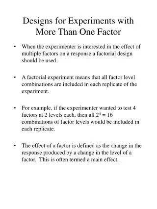
Designs for Experiments with More Than One Factor • When the experimenter is interested in the effect of multiple factors on a response a factorial design should be used. • A factorial experiment means that all factor level combinations are included in each replicate of the experiment. • For example, if the experimenter wanted to test 4 factors at 2 levels each, then all 24 = 16 combinations of factor levels would be included in each replicate. • The effect of a factor is defined as the change in the response produced by a change in the level of a factor. This is often termed a main effect.
20 40 B2 B1 10 30 A1 A2 • Consider the experiment depicted above. Here we have 2 factors each investigated at 2 levels. • The main effect of each factor is calculated as the difference between the average response at the first level of the factor and the average response at the second level of the factor.
It is often useful to graphically display the results of the experiment. Note that we can easily see the effects calculated earlier.
20 0 B2 • This are the results from a similar experiment where factors interact. When the interaction effects are large the main effects have little meaning B1 10 30 A1 A2
General 2k Designs • 2k designs are popular in industry particularly in the exploratory phase of process and product improvement. They consist of k factors each studied at two levels (usually denoted as high and low levels). Our first example was a 22 design. • A simple notation has been developed to represent the replicates. • A run is represented by a series of lowercase letters. If a letter is present it indicates that the corresponding factor is set at its high level. The run with all factors set at their low levels is denoted as (1)
b ab High(+) • This notation applied to our first example is as follows: • The main effect is then just the difference between the average of the observations on the right side of the square and the average of the observations on left side of the square, if n = the number of replicates under each factor combination then the main effect of factor A is: Low(-) (1) a Low(-) High (+)
The main effect of B is the difference between the average of the observations at the top of the square and the average at the bottom of the square: • The interaction effect is found by taking the difference in the diagonal averages: • The terms in the brackets in each of these equations are called contrasts. For example: • ContrastA = a + ab - b - (1) • Note that the coefficients in these contrasts are always = to either -1 or + 1
A table of + and - signs is helpful in determining the sign on each run for developing the contrasts. • The sum of squares for each effect is then as follows: • The total sum of squares is obtained as usual and the error sum of squares can be obtained by subtraction
An Example • A router is used to cut notches in printed circuit boards. The process is in statistical control, the average dimension is satisfactory, but there is too much variability in the process which leads to problems in assembly. The quality improvement team identified two factors which may have an impact: bit size (A) (tested at 1/8 inch and 1/16 inch) and the speed (B) (tested at 40 rpm and 80 rpm). It was felt that vibration of the boards during the process was responsible for the excess variation. An experiment was conducted using four boards at each treatment level. The treatment levels were randomly assigned to the 16 boards and the results are as follows:
Calculate the main and interaction effects and the sum of squares.
Residual Analysis • The residuals from a 2k design are easily obtained through fitting a regression model to the data. For our experiment the appropriate model is as follows: • This model can also be used for obtaining predicted values for the four points in our experimental design.
Minitab Ouput: General Linear Model: Vibration versus A, B Factor Type Levels Values A fixed 2 1 -1 B fixed 2 1 -1 Analysis of Variance for Vibration, using Adjusted SS for Tests Source DF Seq SS Adj SS Adj MS F P A 1 1107.23 1107.23 1107.23 185.25 0.000 B 1 227.26 227.26 227.26 38.02 0.000 A*B 1 303.63 303.63 303.63 50.80 0.000 Error 12 71.72 71.72 5.98 Total 15 1709.83 Term Coef SE Coef T P Constant 23.8313 0.6112 38.99 0.000 A1 8.3188 0.6112 13.61 0.000 B1 3.7688 0.6112 6.17 0.000 A* B 4.3562 0.6112 7.13 0.000
Designs for K 3 • The methods for 22 designs discussed can be easily extended to designs involving more than two factors. The effects are calculated similarly, • As are the sum of squares, • An article in Solid State Technology describes an experiment for improving the etch rate on a wafer plasma etcher. The factors in the experiment were gas flow (A), power applied to the cathode (B), gap between the cathode and the anode (C), and pressure (D). Each factor was tested at two levels. We will assume a single replicate was performed with the following results: • Use Minitab to analyze the results
Fractional Factorial Designs • Since the number of runs increases exponentially with the number of factors investigated in a 2k design it is desirable to limit the number of runs while maintaining the ability to obtain information on the factors of interest. If we can assume that the higher order interactions are negligible, then a fractional factorial design involving fewer than 2k runs may be used. Consider the 23 design matrix depicted below: • Note that in the full factorial design, the sum of the products of any two columns = 0. This indicates that the columns are orthogonal, e.g, their associated effects are statistically independent. • If we were to assume that the high order interaction, ABC were insignificant we might conduct the experiment using just the top half of the design matrix
Notice that the 2(3-1) design is formed by selecting only those runs that yield a + on the ABC effect. The interaction ABC is termed the generator of this fraction. • The estimates of the main effects from this fractional design are as follows A = 1/2 [a - b - c + abc] B = 1/2[-a + b - c + abc] C = 1/2[-a - b + c + abc] also, BC = 1/2[a - b - c + abc] AC = 1/2[-a + b - c + abc] AB = 1/2[-a - b + c + abc] Note that the linear combination of observations in column A estimates A + BC. Therefore, if the contrast is significant, we cannot tell whether it is due to the main effect of A or the interaction effect of B or a mixture of both. That is, the two columns are no longer orthogonal. Two or more effects that have this property are termed aliases. The alias for any factor can be found by multiplying the factor by the generator
The alias of A is: A x ABC = A2BC = BC • likewise, • the alias of B = AC • the alias of C = AB • If we had chosen the other half fraction, the generator would have been -ABC and the aliases would be: • A = -BC • B = -AC • C =-AB • That is the column associated with A really estimates A - BC, the column associated with B estimates B - AC and the column associated with C estimates C - AB • The fraction with the + sign is sometimes referred to as the principle fraction while the fraction with the - sign is termed the alternate fraction.
Using sequences of fractional designs to estimate effects • If we had chosen the first design and were convinced that the two-way interactions were insignificant then the design will produce estimates of the main effects of the three factors. If, however, after running the principle fraction we believe are uncertain as to the interaction effects we can estimate them by running the alternate fraction. • It is easy to construct a 2 k-1 design. Simply write down the treatment levels for the full factorial experiment in k-1 factors. Then equate the column associated with the kth factor with the product of the signs of the k-1 factors. For example we would construct a 24-1 fractional factorial for our plasma etching experiment as follows:
The minitab output below agrees substantially with the output generated from the full factorial design. Factor Type Levels Values A fixed 2 -1 1 D fixed 2 -1 1 Analysis of Variance for response, using Adjusted SS for Tests Source DF Seq SS Adj SS Adj MS F P A 1 32258 32258 32258 71.80 0.001 D 1 168780 168780 168780 375.69 0.000 A*D 1 78012 78012 78012 173.65 0.000 Error 4 1797 1797 449 Total 7 280848 Term Coef SE Coef T P Constant 756.000 7.494 100.88 0.000 A -1 63.500 7.494 8.47 0.001 D -1 -145.250 7.494 -19.38 0.000 A* D -1 -1 -98.750 7.494 -13.18 0.000