Download
1 / 60
700 likes | 1.17k Views
Stream networks and watersheds. The size and land use of the drainage (=catchment) basin is critically important in determining both the quantity and quality of water in a stream. Lakes and ponds are “ lentic ” Streams and rivers are “ lotic ”. Plum Run watershed. Hydrologic Sources.

E N D
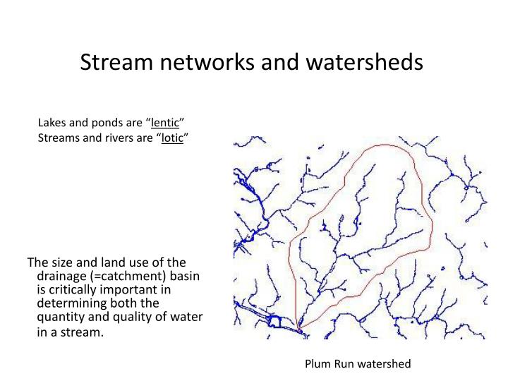
Stream networks and watersheds The size and land use of the drainage (=catchment) basin is critically important in determining both the quantity and quality of water in a stream. Lakes and ponds are “lentic” Streams and rivers are “lotic” Plum Run watershed
Hydrologic Sources • Water enters a stream largely via: • 1. overland runoff (esp. in drainages with steep slopes, much pavement, soils with little permeability or frozen; prominent mostly directly after precipitation events) • 2. groundwater inputs (This is actually a two-way street. “Upwelling” zones are locations where groundwater enters the stream, while water leaves the stream in “downwelling” areas)
Groundwater • Upwelling zones can often be detected by • Unusually cold water of the surface sediments • High conductivity values (high ion content) at the sediment-water interface. • Evidence of high primary production. • Groundwater inputs are much less influenced by short-term variation in precipitation. Limestone stream in Guizhou Province, China
0 Drainage Patterns Stream network patterns reflect the underlying rock and slope topography
Stream Order A first order stream has no tributaries; a 2nd-order stream has 2 1st-order tributaries, a 3rd-order stream has 2 2nd-order tributaries, etc. Which drainage pattern is shown?
Link Magnitude • “The total number of 1st-order source streams upstream of a particular location.” • Streams in this region vary from 1-8 in terms of stream order, but from 1- >1000 in link magnitude. X Give the Stream Order at Site X _____ Give its Link Magnitude ______
Stream Slope • S = (Es - Em )/L • Where E = the elevation at the source • E = the elevation at the mouth • L = the stream length • We calculated this for Lititz Run using Google Earth. • Stream slope is normally steepest near the source • Is this the case in Lanc. Co.? Elev. Distance downstream
Sinuosity The degree of meandering of the stream channel, defined for a given reach as the stream length/valley length.
Width/Depth Ratio An index value which indicates the shape of the channel cross-section (ratio of bank-full width/mean bank-full depth). “Entrenched” streams have low W/D ratios
0 Effects of network position on stream characteristics
0 Velocity • The speed of water movement (e.g., m/sec), determined by • a) the elevational gradient • b) local habitat features (e.g., constrictions, bends) • c) proximity to the substrate • Water velocity directly adjacent to the substrate drops to nearly zero, forming a “boundary layer” inside which erosional force is much reduced (v. important to algae and invertebrates). Microhabitats of low flow velocity (e.g., behind large boulders) are utilized by fish for resting/feeding.
0 Discharge • Def: The volume of water passing a point per unit time (e.g., m3/sec, or cfs). • More important to people (e.g., supply for irrigation, drinking water, sewage dilution, recreation, hydroelectric power, etc.), whereas velocity is more important to stream organisms • May be highly variable over time. USGS monitoring stations on major streams of Chester County.
0 Three Methods of Discharge Measurement 1. Volumetric analysis: Funnel all stream water through a narrow opening into a large container, then determine volume and time interval (minimum duration should be at least 5 sec). Suitable for very small streams.
2. Gauging Station method • Measure the height of water passing through a “weir” (usually permanently installed, with a V-notch). • Once calibrated, the water height is proportional to discharge. • This method is suitable for recording changes in discharge at a fixed location over time)
0 3. Measuring Velocity X Cross-Sectional Area • Pick a location without obstructions and fairly uniform downstream flow, narrow if possible to ensure reasonable current velocity • Divide the width into segments (ca. 5-10 segments). In the center of each, place a current meter at 40% of the distance from bottom to surface (just below mid-depth) and obtain current velocity. • Multiply the velocity by the cross-sectional area of the segment; sum these to obtain total discharge. Pygmy-Gurley Meter
Hydrographs • Def: A graph of changing discharge at a given location over time • The response to storm events can tell a great deal about the capacity of the watershed to absorb rainfall or snowmelt.
0 Response of Discharge to Rain Events • Downstream sites respond more slowly than sites upstream • “Flashy” streams, which empty water rapidly from tributary streams and overland runoff, rapidly reach high peaks (short ascending limb), and rapidly tail off (short descending limb) • Stream channelization, removal of natural vegetation, removal of riparian wetlands all tend to make a stream more flashy • Normal discharge (in the absence of the precipitation event) is termed “baseflow”.
0 Effects of Changing Land Use on Short-term Hydrographs • A and B are the same stream site, measured 20 years apart • Which hydrograph reflects greater development of the watershed? Why? • What is the base flow at time B? 10 Discharge (cfs) 5 A B 1 2 3 Day
0 Flooding Events can be a big issue Mississippi River floods frequently, placing pressure on the ACOE to “do something” Brandywine Ck near Lenape after a Winter Storm
0 Flood Duration Curve • Measures the “storage capacity” of a stream (ability to absorb precipitation with minimal flooding). • Suppose two streams of equal mean discharge:
0 Flood Frequency Curve • Measures the probability of a flood of a given magnitude (P), alternatively expressed as the time in years between such floods (T = 1/P). You need consistent measurements of discharge over many decades to do this. • a. Obtain the largest discharge (e.g., m3/sec or cfs) at the site for each year from USGS records. • b. Rank them (m) from largest(=1) to smallest. • c. Calculate T=[n+1]/m for each year, where n = no. of years • d. Graph each discharge (log scale) against its T value (probability scale). What is the expected maximum discharge of a “10-year flood”? Would a flashier stream have a steeper or less steep slope than the one shown in the graph? You don’t need to know how to calculate this
Sediment Transport • Most streams are “alluvial”, transporting sediments from upstream to downstream • Sediments are transported as “suspended load” (smaller particles up in the water column) or “bedload” (larger particles bouncing along the bottom) • The particle sizes transported are determined by current velocity
Stream Habitats reflect sediment transport • Erosional Habitats • Portions of a stream which routinely have high velocities and lose their smaller sediments • Depositional Habitats • Areas which receive these sediments as current velocity slows • The assemblages of sediment-associated meiofauna, algae, and macroinvertebrates may be very different in the two kinds of habitats.
“Legacy Sediments” • Def: “sediments deposited behind dams in the past; once the dam is breached, these sediments erode rapidly creating present problems of stream water quality.” Mill Pond at Strodes Mill during 1800s (above), and current stream banks on East Branch Plum Run just above the mill pond
Turbidity • Measures the degree of scattering of light in the water column • The actual measurement is in NTU (Nephelometric Turbidity Units). • The measurements can be used: • 1. as an indication of suspended sediment load • 2. as an indication of how rapidly light is attenuated in deeper streams • 3. to infer the probable effects of abrasive sediments on invertebrates and fish • 4. as a correlate with changing discharge at a given location
Habitat Classification Terms reflect Spatial Scale • Stream habitats are hierarchically organized by spatial scale, e.g., into • a) drainage networks • b) stream segments • c) reaches • d) channel units (emphasized here) • e) microhabitats • Channel Units • 1. “riffles” (with fast-moving, turbulent water, heterogeneous gravel or cobble substrate, shallow water depth, steep gradient; erosional habitats) • 2. “runs” (moderate flow velocities, less variation in particle size, little depth variation, less turbulence) • 3. “pools” (deeper, depositional areas with lowered current velocity; may be created by rock or debris dams, eddies)
What Channel Unit is shown? • Probable sediment particle size? • Where in a stream network is it likely to be?
Stream segment of Brandywine Ck • Probable Stream Order? • NPP? • Water Temperature? • Likely sinuosity?
Effects of riparian vegetation(two second-order streams) Effect of riparian forest on • Stream width and depth? • Entrenchment? • Flow velocity? A B
Smaller-scale “microhabitats” reflect current velocity • Where is the current the fastest? • Which microhabitat has the slowest current? • What is the effect of the log?
First-order stream passing through hemlock forest • Water Temperature? • Light? • NPP?
0 Effects of Water Temperature on Stream Biota • Metabolic rates and activity levels • Life history attributes (e.g., lifespan, body size, no. eggs produced) • Distribution, particularly of stenothermal (capable of surviving only a narrow range of temps) species • Oxygen levels (cold water at saturation holds more oxygen than warm water)
0 Oxygen Usually at about 100% saturation for water in riffles. Why? Usually lower in zones of heterotrophic activity (e.g., bacteria, invertebrates) such as leaf packs and within organic sediments Often very high within autotrophic microzone of attached algae on rocks in sunlit areas Oxygen a principal determinant of the distribution of animals in streams Oxygen can be used as a diagnostic tool for detecting organic pollution: Oxygen typically “sags” downstream of effluents adding organic molecules/particles to a stream. Why?
0 Organic Materials in Streams DOM • Dissolved Organic Matter is an important food source for bacteria. Some (usually smaller) molecules are more easily utilized than larger, more refractory compounds. • Leachate from fallen leaves is “allochthonous”, and may “stain” the water, attenuating light and thus limiting primary productivity • Algal exudates are an important source of “autochthonous” DOM • Bacterial communities are finely tuned to the diversity of DOM substrates found in a particular stream; the proportion of DOM consumed by bacteria declines sharply when the community is presented with foreign water from another watershed
0 CPOM • 1. “Coarse Particulate Organic Matter” (particles > 1mm in size), mostly leaves and woody debris • 2. CPOM is colonized (“conditioned”) by fungi and bacteria, and the conditioned material is the principal food source for “shredder” invertebrates. • 3. Leaf packs are also an important microhabitat for a wide range of species (typical of streams with riparian canopy) Leaf pack
FPOM • Produced by decomposition of CPOM • May form by flocculation of DOM, mediated by bacteria, growth and demise of algal cells • May enter the stream as soil particulates (already in FPOM form) • Smaller than CPOM, it is also more easily transported downstream and adds to turbidity • Sediments with high FPOM experience • high rates of sediment metabolism • large diel fluctuations in dissolved oxygen
Nutrient Spiraling • DOM, CPOM and FPOM not only cycle, but are also transported downstream. Thus the cycle becomes a spiral • Spiral length (the downstream distance needed to complete the cycle) = SW + SB where SW = distanced traveled dissolved in the water column and SB = distance traveled as a particle (e.g., as drift).
0 Family Chironomidae • Order Diptera • “Midges” (non-biting gnats) • Highly diverse family • The “rabbits” of aquatic systems (rapid growth rates, eaten by everybody …) • Particular genera associated with lake trophic state
0 Chironomid Identification • Note sclerotized head capsule, C-shaped segmented body, prolegs with hooks • Need to mount head capsule to identify Head capsule of Nanocladius Diversity of chironomid taxa Head capsule of predatory tanypodine larva
0 Chironomus larvae • This genus istypical of eutrophic lakes and streams • often blood-red, with ventral, finger-like “blood gills” for obtaining oxygen (see below) • Live in vertical tubes in the sediments Adult Chironomus
Macrobenthic Life Cycles • Profundal spp. may be univoltine, multivoltine, semivoltine, etc. depending on • temperature • oxygen • trophic state • Wt. per individual inversely related to Density Univoltine life cycle
Benthic Invertebrate Secondary Production • “The amount of invertebrate biomass created per unit time” • may be estimated by regraphing density and wt/indiv • 2o Production is the area under the curve • Often expressed per year P(t1t2) = (Nt1 - Nt2)[(Wt2 - Wt1)/2] + Nt2(Wt2 - Wt1) (this estimates production, e.g., as g/m2/d, for the first of the 3 sections of the above graph; compute the other two sections in analogous fashion)
P/B ratios • Because production is hard to measure, biomass is often used as a surrogate • Is the relationship of secondary production (P) to Biomass (B) a constant regardless of the kind of invertebrate? • Effects on P/B of • Temperature? • Life cycle (voltinism)? • Diet (e.g., algivore, predator)?
Hexagenia • Order Ephemeroptera (mayflies) • build U-shaped tubes in the sediments in sublittoral • Note tusks for building tube • Important role in oxygenating the sediments (undulates body to pull water thru tube) • Characteristic of oligotrophic lakes • Huge hatches a sign of good water quality
Family Tubificidae • Phylum Annelida • Often take over when low oxygen eliminates other taxa such as Hexagenia • Very important to bioturbation, ingesting material below the surface and pooping it out on the sediment surface.
Microbenthos/Meiofauna • Traditionally ignored • Usually operationally defined as animals which pass through a 0.5 mm sieve • Separated with difficulty from the sediments (usually by sugar floatation). • The meiofauna has high P/B and may contribute substantially to the diets of macrobenthos
Bacteria • Bacterial densities peak at the sediment-water interface, reaching densities as high as 1010 cells/g of dry mud. Densities drop off to low values within 5 cm below the mud surface. • Catabolic decomposers • Decomposition is selective • (e.g., proteins, simple sugars) are metabolized rapidly, while refractory compounds are consigned to gradual burial • Anabolic members of the benthic food chain • Convert POC to more nutritious food for protistans, small macroinvertebrates
0 Benthic Macroinvertebrates of Streams • Macroinvertebrates (retained by 500-m sieve) frequently used as bioindicators of stream water quality • Easier to ID than algae • Easier to sample than fish • Temporally more stable than water chemistry • Much higher diversity than in the profundal zone of lakes • Many of the same groups as in the lake littoral • Mollusks, aquatic insects, crocrustacea, oligochaetes • Microinvertebrates (pass through sieve) present but rarely examined (hard to separate from sediments)