Download
1 / 71
710 likes | 737 Views
Explore the enigmatic production of X-rays in massive stars through spectroscopy and solar comparisons, shedding light on stellar wind-shock interactions and potential magnetic influences. Learn about the Sun's X-ray emission and how massive stars challenge conventional wisdom in astrophysics.

E N D
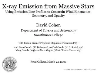
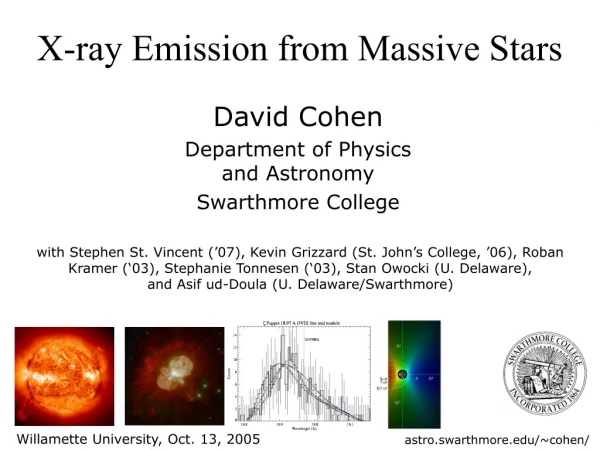
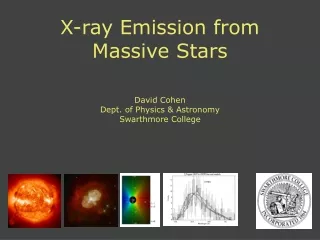
X-ray Emission from Massive Stars David CohenDept. of Physics & AstronomySwarthmore College
X-ray Emission from Massive Stars David CohenDept. of Physics & AstronomySwarthmore College • The work discussed here is with collaborators: • Stan Owocki and Rich Townsend (U. Delaware), Asif ud-Doula (U. Delaware and Swarthmore), Maurice Leutenegger (Columbia), & Marc Gagne (West Chester) • Students: Roban Kramer (’03), Kevin Grizzard (St. John’s College, ’06), Casey Reed (’05), Stephanie Tonnesen (’03), Steve St. Vincent (’07)
X-ray Emission from Massive Stars O and early B stars: M > 8Msun; Teff > 20,000 K; term “massive stars” used interchangeably with “hot stars”
OUTLINE 1. Introduction a. Solar x-ray emission…vs. massive star x-ray emission b. Massive stars and their winds 2. The wind-shock paradigm 3. Chandra spectroscopy of Puppis and Orionis: wind shocks 4. Chandra spectroscopy of 1 Orionis C: signatures of a magnetized wind 5. Conclusions
OUTLINE 1. Introduction a. Solar x-ray emission…vs. massive star x-ray emission b. Massive stars and their winds 2. The wind-shock paradigm 3. Chandra spectroscopy of Puppis and Orionis: wind shocks 4. Chandra spectroscopy of 1 Orionis C: signatures of a magnetized wind 5. Conclusions
X-rays from the Sun • Remember - for thermal radiation - the frequency of light (the energy of each photon) is proportional to the temperature of the emitter: • Human body = 300 K 10 microns, or 100,000 Å (infrared) • Sun, light bulb filament = 6000 K 5000 Å (visible, yellow) • Hot star’s surface = 40,000 K 750 Å (far ultraviolet) • Really hot plasma = 5,000,000 K 6 Å (X-ray) • *don’t forget that thermal emitters give off photons with a range of wavelengths; those listed above represent the peak of the distribution or the characteristic wavelength. Note: an Angstrom unit (Å) is equivalent to 0.1 nanometers (nm)
The Sun is a strong source of X-rays (10-5 of the total energy it emits) It must have ~million degree plasma on it The hot plasma is generally confined in magnetic structures above – but near - the surface of the Sun.
Visible solar spectrum: continuum, from surface X-ray/EUV solar spectrum: emission lines from hot, thin plasma above the surface
We can use spectroscopy - in our study of massive stars (where spatial structure can’t be imaged) - to diagnose plasma kinematics (via Doppler-broadened line shapes) and plasma location with respect to the stellar surface (via UV-sensitive line ratios) Theme: spectroscopy as a proxy for imaging. X-ray/EUV solar spectrum: emission lines from hot, thin plasma above the surface
This hot plasma is related to magnetic fields on the Sun: confinement, spatial structure, conduits of energy flow, heating
More magnetic structures on the Sun: x-ray image from TRACE
The Sun’s magnetic dynamo requires rotation + convection to regenerate and amplify the magnetic field Note granulation, from convection Sunspots over several days: rotation
OK, so the Sun emits x-rays - quite beautifully - and they’re associated with its magnetic activity, related to convection and rotation… But what of hot, massive stars?
OUTLINE 1. Introduction a. Solar x-ray emission…vs. massive star x-ray emission b. Massive stars and their winds 2. The wind-shock paradigm 3. Chandra spectroscopy of Puppis and Orionis: wind shocks 4. Chandra spectroscopy of 1 Orionis C: signatures of a magnetized wind 5. Conclusions
Hot, Massive Stars Stars range in (surface) temperature from about 3500 K to 50,000 K Their temperatures correlate with mass and luminosity (massive stars are hot and very bright): a 50,000 K star has a million times the luminosity of the Sun (Tsun = 6000 K) Stars hotter than about 8000 K do not have convective outer layers - no convection - no dynamo - no hot corona… …no X-rays ?
Our Sun is a somewhat wimpy star… zPuppis: 42,000 K vs. 6000 K 106 Lsun 50 Msun
Optical image of the constellation Orion Note: many of the brightest stars are blue (i.e. hot, also massive)
In 1979 the Einstein Observatory made the surprising discovery that many O stars (the hottest, most massive stars) are strong X-ray sources Chandra X-ray image of the Orion star forming region q1Ori C: a 45,000 K O-type star Note: X-rays don’t penetrate the Earth’s atmosphere, so X-ray telescopes must be in space
So, we’ve got a good scientific mystery: how do massive stars make X-rays? Could we have been wrong about the lack of a magnetic dynamo - might massive star X-rays be similar to solar X-rays? Before we address this directly, we need to know about one very important property of massive stars (that might provide an alternate explanation for their X-rays)…
Massive stars have very strong radiation-driven stellar winds What is a stellar wind? It is the steady loss of mass from the surface of a star into interstellar space The Sun has a wind (the “solar wind”) but the winds of hot stars can be a billion times as strong as the Sun’s Hubble Space Telescope image ofhCar; an extreme example of a hot-star wind
How do we know these hot-star winds exist? Spectroscopy! rest wavelength(s) – this N V line is a doublet Absorption comes exclusively from region F - it’s all blue-sifted You can read the terminal velocity (in km/s) rightoff the blue edge of the absorption line bluewavelengthred
Why do hot star winds exist? The solar wind is actually driven by the gas pressure of the hot corona But hot-star winds are driven by radiation pressure Remember, photons have momentum as well as energy: And Newton tells us that a change in momentum is a force:
So, if matter (an atom) absorbs light (a photon) momentum is transferred to the matter Light can force atoms to move! re, the radius of an electron, giving a cross section,sT(cm2) The flux of light, F (ergs s-1 cm-2) The rate at which momentum is absorbed by the electron By replacing the cross section of a single electron with the opacity (cm2 g-1), the combined cross section of a gram of plasma, we get the acceleration due to radiation
For a (very luminous) hot star, this can compete with gravity…but note the 1/R2 dependence, if arad > agrav, a star would blow itself completely apart. And free electron opacity, and the associated Thompson scattering, can be significantly augmented by absorption of photons in spectral lines – atoms act like a resonance chamber for electrons: a bound electron can be ‘driven’ much more efficiently by light than a free one can (i.e. it has a much larger cross section), but it can only be driven by light with a very specific frequency.
Radiation driving in spectral lines not only boosts the radiation force, it also solves the problem of the star potentially blowing itself apart: As the radiation-driven material starts to move off the surface of the star, it is Doppler-shifted, making a previously narrow line broader, and increasing its ability to absorb light. cont. 0 Optically thick line – from stationary plasma (left); moving plasma (right) broadens the line and increases the overall opacity.
The Doppler desaturation of optically thick (opaque) lines allows a hot-star wind to bootstrap itself into existence! And causes the radiation force to deviate from strictly 1/R2 behavior: the radiation force on lines can be less than gravity inside the star but more than gravity above the star’s surface.
OUTLINE 1. Introduction a. Solar x-ray emission…vs. massive star x-ray emission b. Massive stars and their winds 2. The wind-shock paradigm 3. Chandra spectroscopy of Puppis and Orionis: wind shocks 4. Chandra spectroscopy of 1 Orionis C: signatures of a magnetized wind 5. Conclusions
X-rays from shock-heating in line-driven winds The Doppler desaturation that’s so helpful in driving a flow via momentum transfer in spectral lines is inherently unstable The line-driven instability (LDI) arises when a parcel of wind material is accelerated above the local flow speed, which moves it out of the “Doppler shadow” of the material behind it, exposing it to more photospheric radiation, and accelerating it further…
Numerical modeling of the hydrodynamics show lots of structure: turbulence, shock waves, collisions between “clouds” This chaotic behavior is predicted to produce X-rays through shock-heating of some small fraction of the wind.
A snapshot at a single time from the same simulation. Note the discontinuities in velocity. These are shock fronts, compressing and heating the wind, producing x-rays. There are dense inter-shock regions, though, in which cold material provides a source of photoelectric absorption
Even in these instability shock models, most of the wind is cold and is a source of x-ray continuum opacity - x-rays emitted by the shock-heated gas can be absorbed by the cold gas in the rest of the wind Keep this in mind, because it will allow us to learn things about the physical properties of a shocked wind via spectroscopy
X-ray line profiles can provide the most direct observational constraints on the x-ray production mechanism in hot stars Wind-shocks : broad lines Magnetic dynamo : narrow lines The Doppler effect will make the x-ray emission lines in the wind-shock scenario broad, compared to the x-ray emission lines expected in the coronal/dynamo (solar-like) scenario
OUTLINE 1. Introduction a. Solar x-ray emission…vs. massive star x-ray emission b. Massive stars and their winds 2. The wind-shock paradigm 3. Chandra spectroscopy of Puppis and Orionis: wind shocks 4. Chandra spectroscopy of 1 Orionis C: signatures of a magnetized wind 5. Conclusions
So, this wind-shock model - based on the line-force instability - is a plausible alternative to the idea that hot star x-rays are produced by a magnetic dynamo This basic conflict is easily resolved if we can measure the x-ray spectrum of a hot star at high enough resolution… In 1999 this became possible with the launch of the Chandra X-ray Observatory
Mg XII • Pup (O4 I) Si XIV Ne X Fe XVII Ne IX O VIII O VII N V 10 Å 20 Å
Focus in on a characteristic portion of the spectrum 12 Å 15 Å • Pup (O4 I) Capella - a cooler star: coronal/dynamo source Fe XVII Ne X Ne IX
Differences in the line shapes become apparent when we look at a single line (here Ne X Lya) lab/rest wavelength The x-ray emission lines in the hot starzPup are broad -- the wind shock scenario is looking good! But note, the line isn’t just broad, it’s also blueshifted and asymmetric… • Pup (O4 I) Capella (G2 III)
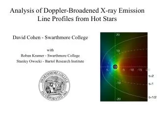
We can go beyond simply wind-shock vs. coronal: We can use the line profile shapes to learn about the velocity distribution of the shock-heated gas and even its spatial distribution within the wind, as well as learning something about the amount of cold wind absorption (and thus the amount of cold wind).
What Line Profiles Can Tell Us • The wavelength of an emitted photon is proportional to the line-of-sight velocity: • Line shape maps emission at each velocity/wavelength interval • Continuum absorption by the cold stellar wind affects the line shape • Correlation between line-of-sight velocity and absorption optical depth will cause asymmetries in emission lines The shapes of lines, if they’re broad, tells us about the distribution and velocity of the hot plasma in the wind -- maybe discriminate among specific wind shock models/mechanisms
We will now build up a physical – but flexible – empirical x-ray emission line profile model: Accounting for the kinematics of the emitting plasma (and the associated Doppler shifting/broadening); Radiation transport (attenuation of the line photons via bound-free absorption in the cold wind component). Note that our line-profile model, while physical, is agnostic regarding the heating mechanism.
Emission Profiles from a Spherically Symmetric, Expanding Medium A spherically-symmetric, x-ray emitting wind can be built up from a series of concentric shells. Occultation by the star removes red photons, making the profile asymmetric A uniform shell gives a rectangular profile.
Continuum Absorption Acts Like Occultation Contours of constant optical depth (observer is on the left) blue red wavelength Red photons are preferentially absorbed, making the line asymmetric: The peak is shifted to the blue, and the red wing becomes much less steep.
Ro=1.5 The model has four parameters: for r>Ro Ro=3 where The line profile is calculated from: Ro=10 Increasing Ro makes lines broader; increasingt*makes them more blueshifted and skewed. t=1,2,4
t=1,2,4 A wide variety of wind-shock properties can be modeled Ro=1.5 Line profiles change in characteristic ways witht*and Ro, becoming broader and more skewed with increasingt*and broader and more flat-topped with increasing Ro. Ro=3 Ro=10
In addition to the wind-shock model, our empirical line-profile model can also describe a corona With most of the emission concentrated near the photosphere and with very little acceleration, the resulting line profiles are very narrow.
We fit all the unblended strong lines in the Chandra spectrum ofzPup: all the fits are statistically good Ne X 12.13 Å Fe XVII 15.01 Å Fe XVII 16.78 Å N VII 24.78 Å Fe XVII 17.05 Å O VIII 18.97 Å
We place uncertainties on the derived model parameters lowest t* best t* highest t* Here we show the best-fit model to the O VIII line and two models that are marginally (at the 95% limit) consistent with the data; they are the models with thehighestandlowestt*values possible.
Lines are well fit by our three parameter model:zPup’s x-ray lines are consistent with a spatially distributed, spherically symmetric, radially accelerating wind scenario, with reasonable parameters: • t*~1 :4 to 15 times less than predicted • Ro~1.5 • q~0 • But, the level of wind absorption is significantly below what’s expected. • And, there’s no significant wavelength dependence of the optical depth (or any parameters).