Download
1 / 10
100 likes | 280 Views
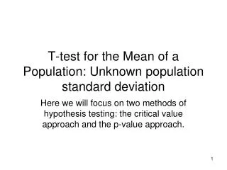
T-test for the Mean of a Population: Unknown population standard deviation. Here we will focus on two methods of hypothesis testing: the critical value approach and the p-value approach.

E N D
T-test for the Mean of a Population: Unknown population standard deviation Here we will focus on two methods of hypothesis testing: the critical value approach and the p-value approach.
We saw in the standard deviation in the population known case that when we do not know the true value of the population mean for a quantitative variable an hypothesis test can be carried out utilizing the z calculation (x bar minus mu under Ho:)/standard error of the mean. When the population standard deviation, sigma, of the variable is unknown we have to rely on the t distribution. Plus in the calculation of the standard error we will use the sample standard deviation. The t statistic = (x bar minus mu under Ho:)/ standard error of the mean. Let’s work a few problems.
Example For a company when they look at the past they have seen the average dollar amount on an invoice be $120. Over time this will be monitored and they will see if this changes. The question now is about whether or not the population mean is still 120. We will make this the null hypothesis. So we have Ho: μ = 120 and H1: μ≠ 120 a) With the critical value approach the value of alpha has to be determined and say we have alpha = .05. When the alternative hypothesis has a not equal to sign we have a two tail test. This means we have .025 in each tail. But since we do not know the population standard deviation we have to use the t distribution. With a sample size of 12 we look in the df = n – 1 = 12 – 1 = 11 row. The critical t’s are thus -2.2010 and 2.2010. Let’s see what this looks like in a graph on the next slide
.025 alpha/2 = .025 lower Critical t = -2.2010 Upper Critical t = 2.2010 Let’s review what we have done. We have a null and alternative hypothesis. We have an alpha value and a sample size we will use. The critical values of t break up the t distribution into rejection and acceptance of the null hypothesis regions. Our decision rule will be this: If when we take a sample and calculate both a sample mean and the associated t value, called the t test statistic (and I will write tstat), if the tstat is less than the lower critical value or greater than the upper critical value we will reject the null. If the tstat is in the middle of the critical values we do not reject the null.
Now say we get an actual sample of 12 invoices and we see the sample mean is 112.85 and the sample standard deviation is 20.80. The tstat from the sample is (112.85 – 120)/(20.804/sqrt(12)) = - 1.19. Since the value of the tstat is -1.19 and since this value is in the middle of the critical values we do not reject the null. b) To proceed with the p-value approach to hypothesis testing I would like us to explore the t distribution with df = 11 row. Let’s see this on the next slide.
T distribution with DF = 11 .25 is area under curve .10 is area under curve .05 is area under curve .025 is area under curve .01 is area under curve .005 is area under curve -3.1058 -2.7181 -2.2010 -1.7959 -1.3634 -0.6974 .0.6974 1.3634 1.7959 2.2010 2.7181 3.1058 Here I have marked off on the t distribution the positive and negative values. On the next slide I reproduce this with the tails colored in for when alpha is picked to be .05.
T distribution with DF = 11 .25 is area under curve .10 is area under curve .05 is area under curve .025 is area under curve .01 is area under curve .005 is area under curve -3.1058 -2.7181 -2.2010 -1.7959 -1.3634 -0.6974 .0.6974 1.3634 1.7959 2.2010 2.7181 3.1058 So, with alpha = .05 the critical t’s are -2.2010 and 2.2010. Next we take the sample mean and calculate the tstat. Again, in our example we had -1.19. The -1.19 occurs here on the number line. This falls between -1.3634 and -.06974. The tail areas for these two values are 0.10 and 0.25, respectively. 7
The tail area for -1.19 is thus between 0.10 and 0.25. This is the basis for the p-value. But, because of the way the t distribution shows up in our book the best we can say about the tail area for the tstat is between 0.10 and 0.25. Since our alternative hypothesis H1 is a not equal to sign we have to double the tail area for -1.19 and so we say the p-value is between 0.20 and 0.50. (A computer or better table would have us see the tail area doubled would be .259 – we do not need that here.) Here is how we use the p-value approach. If the p-value is less than or equal to alpha reject the null, otherwise do not reject the null. In our example the p-value is at least 0.20 which is > .05 so we do not reject the null.
Say from a problem we see Ho: μ = 50 and thus H1: μ≠50. Also say x bar = 56 and s = 12. The tstat = (56 – 50)/(12/sqrt16) = 2.00 On the next slide I show what the critical t’s would be in this problem if we wanted an alpha = .10. Note with n = 16 the df = 15.
alpha = .10/2 Critical t = 1.7531 -1.7531 The critical values of t are -1.7531 and 1.7531. If our tstat is outside these two values then we are saying that the sample information is placing us in a low probability area. This makes us suspicious of the null hypothesis and thus we reject it. Our tstat = 2.00 places us in the rejection region. Note if alpha was .05 we would not reject the null (critical values of – and + 2.1315). The p-value is thus between .05 and .10.