Download
1 / 22
220 likes | 418 Views
Do cloud microphysical parameters derived from daytime multi-spectral satellite observations correlate with rainfall estimates?. Elsa Cattani, Francesca Torricella, and Vincenzo Levizzani ISAC CNR (Italy) Institute of Atmospheric Sciences and Climate National Research Council - Bologna.

E N D
Do cloud microphysical parameters derived from daytime multi-spectral satellite observations correlate with rainfall estimates? Elsa Cattani, Francesca Torricella, and Vincenzo Levizzani ISAC CNR (Italy) Institute of Atmospheric Sciences and Climate National Research Council - Bologna
Outline • Methods used to analyse the cloud and rain fields • Geographic area and time period • The data • Comparison of TMI and PR rain derived products • The RGB microphysical visualization of the cloud field • Retrieval of cloud properties by means of CAPCOM • Compare cloud microphysics & rain • Conclusions
Methods of analysis of the cloud/rain field • Use of the TRMM payload to analyse the cloud/precipitation field in different spectral regions • Exploit TMI & PR operational rainproducts • Consider the PR rain field as the truth and statistically compare the rain data (instantaneous rain intensity at the ground in mm h -1) • Derive the cloud mask from multi-spectral observations for the scenarios • Display RGB pictures of the cloud field derived by combining VIS-NIR and IR channels of the VIRS • Derive cloud microphysical parameters by means of a suitable retrieval scheme (CAPCOM) • Produce & compare the maps
Study area and period • West Africa (WA) • - 5 < LAT < 20 - 25 < LON < 25 • June 2004 (from 1th to 10th) • Area characterized byclusters of convective precipitation or MCSs • Convection tends to initiate in the lee of mountains and propagates in general direction of prevailing flow • Convection can regenerate through a number of diurnal cycles
TRMM operational products used in the analysis (from GES DAAC) http://daac.gsfc.nasa.gov/www/ post-boost
Examples of rain maps from PR and TMI June 1st, daytime (i.e. SZA < 70°) mm h-1
Statistical comparison of TMI and PR surface rain data desertic arid dlat =0.1° sea wet dlon =0.1° • The original 2A12 and 2A25 rain data are mapped to 0.1° latitude –longitude grid. On average 20 PR and 27 TMI observations in each grid mesh • Daytime data: 40 orbits for TMI (34,462 pixels in the common area of the swaths) and 35 PR orbits (108,406 pixels) over the area during the 10 days • The rain information from PR and TMI are compared after re-projection onto this grid • The whole WA is divided in macro-areas • For each macro-area the analysis is applied separately • The PR 2A25 rain data are considered as rain truth data
Definitions from: WWRP/WGNE Joint Working Group on Verification Forecast Verification - Issues Probability of detection (hit rate)* Answers the question: What fraction of the observed "yes" events were correctly forecast? Range: 0 to 1. Perfect score: 1. False alarm ratio Answers the question: What fraction of the predicted "yes" events actually did not occur (i.e., were false alarms)? Range: 0 to 1. Perfect score: 0. Heidke skill score (Cohen's k) where Answers the question: What was the accuracy of the forecast relative to that of random chance? Range: minus infinity to 1, 0 indicates no skill. Perfect score: 1. * We used both POD0 i.e. having a zero rain/no-rain boundary and POD1, having 1 mm h-1 rain/no-rain boundary
Table of Statistics bad good
RGB display of VIRS measurements The RGB technique provides a relatively simple rendering of multispectral satellite information for the meteorological scenario interpretation The optimum coloring of the RGB image composites rely on the proper selection of thechannels and the enhancement of the individual colors The channel selection must be driven by the particular phenomenon (low or high clouds, dust, smoke etc.) to be emphasized in the satellite image The proper color enhancement requires the conversion from radiances to brightness temperatures (IR channels) or reflectances (VIS/NIR channels), selection of the display mode (inverted or not inverted), stretching of the dynamic range of the satellite data, and gamma correction The adopted scheme, so-called day microphysical is particularly recommended for cloud analysis (optical thickness, effective size and top height) and for emphasizing the presence of severe convection
Adopted RGB display: “day microphysical” From the SEVIRI images interpretation guidelines*, we selected the so-called day-microphysical scheme, developed to interpret and analyze the following components/scenarios: Cloud – Convection – Fog – Snow – Fires Adapted to VIRS, it combines channels this way: R = Channel 01 (VIS0.6) G = Channel 03 (NIR3.7 only reflected solar component) B = Channel 04 (IR10.8) June 1th deep precip cloud thin Cirrus small ice particle thin Cirrus large ice particle severe conv. ocean veget. land * By, and with the contribution of: H. P. Roesli, J. Kerkmann, D. Rosenfeld, M. König Available at http://oiswww.eumetsat.org/WEBOPS/msg_interpretation/index.html
Identifying the cloudy pixels The cloud mask can be described as a cascade of tests involving VIRS channels. It is applied separately over land and sea pixels. Cloudy pixel in the cloud swath are identified by using very conservative tests, already set to identify precipitating clouds by the CERES science team. This kind of selection identify optically thick, ice clouds such as towering cumulonimbus. Over the land if [TB(CH4) < 257 K] and [R(CH1) > 0.38] it’s a cloud and also [TB(CH3) - TB(CH4) > 20 K] and [TB(CH4) < 237 K] and [R(CH1) > 0.45] it’s raining (maybe!) Over the sea First avoid sun glint: θscatt> 36° then if [TB(CH4) < 257 K] and [R(CH1) > 0.065] it’s a cloud and also [TB(CH3) - TB(CH4) > 20 K] and [TB(CH4) < 237 K] and [R(CH1) > 0.45] it’s raining (maybe!)
Example of cloud mask map June 1st thick cloudraining cloud
Microphysical properties retrieval from VIRS: CAPCOM (Comprehensive Analysis Program for Cloud Optical Measurement) • It allows for the retrieval of cloud optical thickness (), effective radius (Re) and top temperature (Ttop) from satellite measurements in the VIS, NIR and IR channels. The cloud phase is supposed known. • Undesirable radiation components (ground reflected and thermal emitted radiation, NIR thermal contribution) are subtracted from the satellite radiance to derive the cloud signal. • The retrieval is performed by means of comparison between the modelled cloud radiances and the corresponding satellite radiance measurements. • The LUTs are built for a grid of selected values of , Re, Ttop, water vapour amount above and below the cloud layer, solar zenith, satellite zenith and relative azimuth angles. Separate LUTs for ice and water clouds are computed. Nakajima, T. Y., and T. Nakajima, 1995, J. Atmos. Sci.,52, 4043 – 4059 Kawamoto, K., T. Nakajima, and T. Y. Nakajima, 2001, J. Climate, 14, 2054 – 2068 CAPCOM is available at http://www.ccsr.u-tokyo.ac.jp/~clastr/
CAPCOM flow chart Simulated radiances FIRST GUESS of c, Re, Tc Current values of c, Re, Tc Ancillary data AD T(z), WV(z), P(z) Computes Z e PC i-th iteration Observing geometry Computes LWP, LWC and D Computes WeuWecWel LUTS Corrects measurements Measured radiances LRTM(0.6) LRTM(3.7) LRTM (11) LSR LTHC LTHG LTHU LTHL indesiderable components to be removed from measurements [LCORR() - LRTM()]/LCORR() i 10 Newton-Raphson method Check the convergence c, Re, Tc retrieved = current values Compute new current values for c, Re, Tc yes no i > 10: re-computes first guess
180 60 40 30 20 14 5 µm Case 1: June 1st, orbit #37307, LT ~ 13:20, rain over the ocean Effective radius RGB + PR Cloud mask PR TMI
180 60 40 30 20 14 5 µm Case 2: June 1th, orbit #37306, LT ~ 13:15, rain over land Cloud mask RGB + PR TMI PR
180 60 40 30 20 14 5 µm Case 3: June 3th, orbit #37337, LT ~ 12:40, rain over the coast RGB + PR Cloud mask Effective radius TMI PR
Conclusions (1/2) • Based on TRMM data, WA daytime convection is analysed in several channels (from VIS to MW) to derive maximum information on rain processes • Cloud mask tests perform very well in this geographic area having such large thermal contrast between cloud top and surface • Cloud structures delineated in the cloud mask nicely agree with RGB images • Rain data derived from TMI and PR show a limited agreement depending also on the climatic sub-area, due to differences in algorithms, resolution, observing geometry, frequency, etc.
Conclusions (2/2) • The microphysical characterization of the cloud tops (especially in terms of Re) does not add significant information about the underlying precipitation layer: the thick frozen layer detected from the scattering in TMI high frequency channels is detected in multispectral VIRS data as well, but even the greater Re values do not correlate with surface rain • Moreover, due to the input set-up of the microphysical retrieval code, in large areas corresponding to the colder and higher (overshooting) cloud structure, the algorithm is not able to retrieve meaningful information, probably due to the very low temperatures, not represented in the input data and the vanishing sensitivity of the 3.7 µm reflectances to Re • The cloud mask from VIRS channels, can be considered a useful input to the screening procedure of PMW based rain algorithm
Scan angle ± 65° Scan angle ± 17° Scan angle ± 45° Frequency 10.65 GHz 19.35 GHz 21.3 GHz 37.0 GHz 85.5 GHz Polarization V & H V & H V V & H V & H Frequency 13.8 GHz Wavelenghts 0.623 μm 1.610 μm 3.784 μm 10.826 μm 12.028 μm Instruments onboard TRMM TMI PR VIRS