Download
1 / 20
200 likes | 218 Views
OCO provides spatially resolved spectroscopic observations of CO2 and O2 to identify sources and sinks, monitoring CO2 fluxes on regional scales. Learn about the OCO mission architecture, precise measurements, and anticipated data products.

E N D
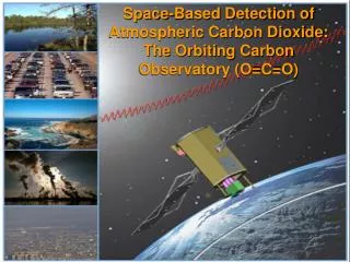
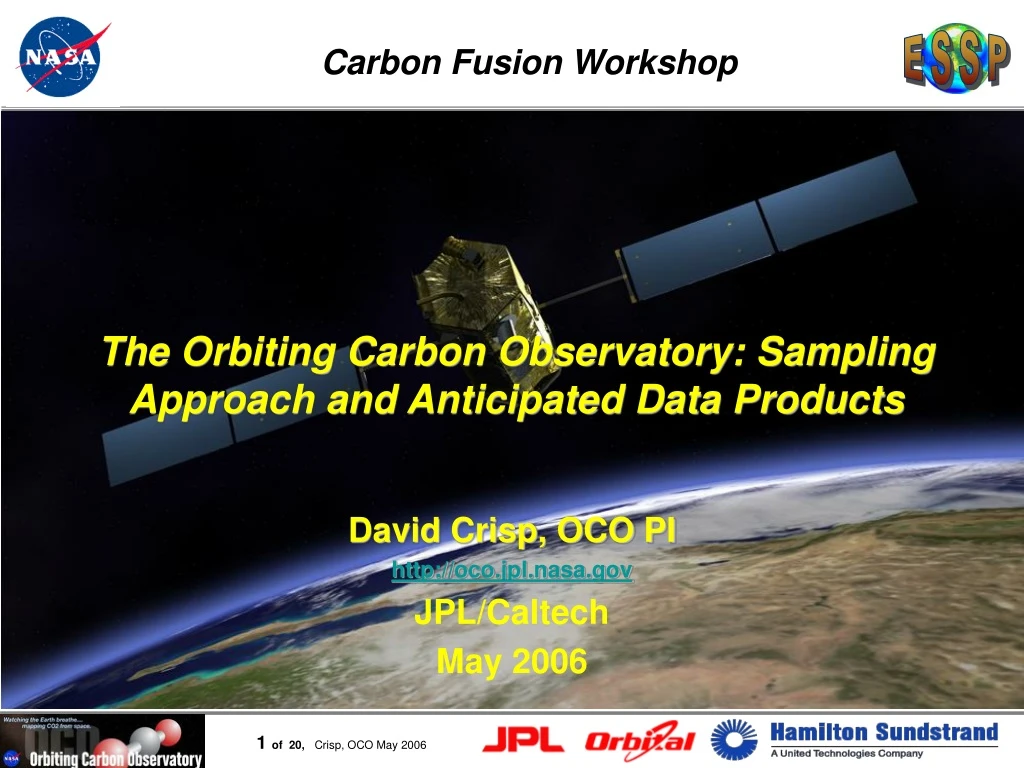
Carbon Fusion Workshop The Orbiting Carbon Observatory: Sampling Approach and Anticipated Data Products David Crisp, OCO PI http://oco.jpl.nasa.gov JPL/Caltech May 2006
C O O What Processes Control Atmospheric CO2? Carbon dioxide (CO2) is the: Main atmospheric component of the global carbon cycle Main man-made greenhouse gas Only half of the CO2 produced by human activities is remaining in the atmosphere
Outstanding Questions • Where are the sinks that are absorbing almost 50% of the CO2 that we emit? • Land or ocean? • Eurasia/North America? • Why does CO2 buildup vary dramatically with nearly uniform emissions? • How will CO2 sinks respond to climate change?
The Orbiting Carbon Observatory (OCO) OCO will acquire the space-based data needed to identify CO2 sources and sinks and quantify their variability over the seasonal cycle Approach: • Collect spatially resolved, high resolution spectroscopic observations of CO2 and O2 absorption in reflected sunlight • Use these data to resolve spatial and temporal variations in the column averaged CO2 dry air mole fraction,XCO2over the sunlit hemisphere • Employ independent calibration and validation approaches to produce XCO2 estimates with random errors and biases no larger than 1 - 2 ppm (0.3 - 0.5%) on regional scales at monthly intervals
Precise Measurements Needed to Constrain CO2 Surface Fluxes • Resolve pole to pole XCO2 gradients on regional scales • Resolve the XCO2 seasonal cycle in the Northern Hemisphere 364 Precisions of 1–2 ppm (0.3–0.5%) on regional scales needed to: • Resolve (8ppm) pole to pole XCO2 gradients on regional scales • Resolve the XCO2 seasonal cycle in the Northern Hemisphere 356
OCO Fills a Critical Measurement Gap 6 NOAA TOVS 5 Aqua AIRS 4 ENVISAT SCIAMACHY 3 CO2 Error (ppm) 2 Aircraft 1 Flask Site Globalview Network OCO Flux Tower 0 1000 10000 1 100 10 Spatial Scale (km) OCO will make precise global measurements of XCO2 over the range of scales needed to monitor CO2 fluxes on regional to continental scales.
CO2 2.06 m CO2 1.61m O2 A-band Clouds/Aerosols, Surface Pressure Column CO2 Clouds/Aerosols, H2O, Temperature Making Precise CO2 Measurements from Space • High resolution spectra of reflected sunlight in near IR CO2 and O2 bands used to retrieve the column average CO2 dry air mole fraction, XCO2 • 1.61 m CO2 bands – Column CO2 with maximum sensitivity near the surface • O2 A-band and 2.06 m CO2 band • Surface pressure, albedo, atmospheric temperature, water vapor, clouds, aerosols • Why high spectral resolution? • Enhances sensitivity, minimizes biases
Glint Spot Ground Track Local Nadir OCO Observing Strategy • Nadir Observations: tracks local nadir • + Small footprint (< 3 km2) isolates cloud-free scenes and reduces biases from spatial inhomogeneities over land • Low Signal/Noise over dark ocean • Glint Observations: views “glint” spot • + Improves Signal/Noise over oceans • More interference from clouds • Target Observations • Tracks a stationary surface calibration site to collect large numbers of soundings • Data acquisition schedule: • alternate between Nadir and Glint on 16-day intervals • Acquire ~1 Target observation each day
1:18 OCO Will Fly in the A-Train Coordinated Observations CloudSat – 3-D cloud climatology CALIPSO – 3-D aerosol climatology aerosols, polarization AIRS – T, P, H2O, CO2, CH4 MODIS – cloud, aerosols, albedo TES – T, P, H2O, O3, CH4, CO MLS – O3, H2O, CO HIRDLS – T, O3, H2O, CO2, CH4 OMI – O3, aerosol climatology OCO - - CO2 O2 A-band ps, clouds, aerosols • OCO files at the head of the A-Train, 12 minutes ahead of the Aqua platform • 1:18 PM equator crossing time yields same ground track as AQUA • Near noon orbit yields high SNR CO2 and O2 measurements in reflected sunlight • CO2 concentrations are near their diurnally-averaged values near noon • Maximizes opportunities of coordinated science and calibration activities
Mission Architecture Project Management (JPL) • Science & Project Team • Systems Engineering, Mission Assurance • Ground Data System Single Instrument (Hamilton Sundstrand) • 3 high resolution grating spectrometers Dedicated Bus (Orbital Sciences) • LEOstar2: GALEX, SORCE, AIM Dedicated Launch Vehicle (Orbital Taurus 3110) • September 2008 Launch from Vandenberg AFB Mission Operations (JPL/Orbital Sciences) • NASA Ground Network, Poker Flats, Alaska
The OCO Instrument • 3 bore-sighted, high resolution, grating spectrometers • O2 0.765 m A-band • CO2 1.61 m band • CO2 2.06 m band • Similar optics and electronics • Common 200 mm f/1.9 telescope • Spectrometers cooled to < 0 oC • Resolving Power ~18,000/21,000 • Common electronics for focal planes • Existing Designs For Critical Components • Detectors: WFC-3, Deep Impact (RSC) • Cryocooler: TES flight spare (NGST)
Prevailing Winds OCO Sampling over a 16-Day Repeat Cycle Space-based CO2 column measurements complement surface measurement network. OCO 3-Days • OCO Sampling Rate/Coverage • 12-24 samples/second collected along track over land and ocean • Glint: +75o SZA • Nadir: +85o SZA • Longitude resolution 1.5o OCO 1-Day OCO Sampling: Clouds reduce number of usable samples Chevallier et al. 2006
OCO Data Hierarchy Spatial Spectrum Spectral 1 2 Pixel 5 Sounding: 3 Collocated Spectra 3 Granule: All ~30,000 Soundings recorded each orbit Frame: 4 (8) Cross-Track Soundings 4
Averaging Kernels: Early Support for Source/sink inversions OCO characterization for Key Environmental Parameters (SZA, surface type) • Study effect on XCO2 biases on CO2 source/sink inversions • Rehearsal of ingesting OCO XCO2 (early feedback on L2 product)
Example: XCO2 Averaging Kernel and Errors for a Single Orbit Track Single Sounding XCO2 Errors Nadir Viewing Averaging Kernel Along Orbit Track
Spatial/Temporal Sampling Constraints MISR Aerosol Factors Limiting Sampling Density • Orbit ground track • Clouds and Aerosols • OCO can collect usable samples only in regions where the cloud and aerosol optical depth < 0.3 • Low Surface Albedo • Others? MODIS Cloud
Space-based XCO2 Validation Strategy • The space-based XCO2 data will be validated against the surface WMO standard for CO2 using measurements of XCO2 from ground based Fourier transform spectrometers (FTS) as a transfer standard • XCO2 will be retrieved from the FTS and space-based instruments using same retrieval code • FTS XCO2 compared to: • Surface in situ CO2 • Tall tower in situ CO2 • Column CO2 integrated from in situ profiles • FTS XCO2 performance tracked by monitoring: • Instrument Line Shape (HCl gas cell) • Pointing (Doppler shift, telluric vs solar features) • XO2, surface pressure and H2O WLEF FTIR Observations at 79°N (Spitsbergen) FTS Notholt et al., GRL, 2005 Observations at 79°N (Spitsbergen) FTS Notholt et al., GRL, 2005
Summary of Data Products • Four major products • Level 0 – Time-ordered science and housekeeping data • Raw data, excluding spacecraft packet information for data transfer to ground • Level 1A - Parsed and merged science and instrument housekeeping telemetry • Data subdivided into discretely named elements • Data from all three spectrometers correlated in a single frame • Corresponding temperature and voltage measures from housekeeping merged into appropriate frame • Level 1B - Spatially ordered, Geolocated, calibrated spectra • Level 2 - Geolocated retrieved state vectors with column averaged CO2 dry air mole fraction
OCO Data Product Volumes • The above estimates assume that the GDS retains just a single copy of each data product • If multiple versions of the data are maintained, the estimated volume required for OCO products could exceed 30 TBytes. • Level 2 Product volume reflects the size of the distributable product • Additional “expert products: will be generated for OCO Science team use will require an additional ~55.7 Gbytes per orbit, or about 0.79 Gbytes per day
OCO Schedule • 7/2001: Step-1 Proposal Submitted • 2/2002: Step-2 Proposal Submitted • 7/2003: Selected for Formulation • 7/2004: System PDR • 5/2005: Mission Confirmed for Implementation • 10/2005: Instrument CDR • 2/2006: Spacecraft CDR • 7/2006: MOS/GDS CDR • 8/2006: System CDR • 2-4/2007: Instrument Testing • 5/2007: Instrument Delivery to SC • 10/2007: Observatory Integration begins • 6/2008: Launch Vehicle Integration begins • 9/2008: Launch from VAFB • 10/2010: End of Nominal Mission < ESA 3rd Party Mission