Download
1 / 19
190 likes | 276 Views
Understanding Optimal Interpolation (OI) for spatial data, assessment of forecast errors, and the application of EnKF for ensemble-based corrections in atmospheric modeling.

E N D
Advanced data assimilation methods-EKF and EnKF Hong Li and Eugenia Kalnay University of Maryland 17-22 July 2006
Recall the basic formulation in OI • OI for a Scalar: Optimal weight to minimize the analysis error is: • OI for a Vector: • B is statistically pre-estimated, and constant with time in its practical implementations. Is this a good approximation? t=0 t=6h True atmosphere
OI and Kalman Filter for a scalar • OI for a scalar: • Kalman Filter for a scalar: • Now the background error variance is forecasted using the linear tangent model L and its adjoint LT
“Errors of the day” computed with the Lorenz 3-variable model: compare with rms (constant) error =0.08 • Not only the amplitude, but also the structure of B is constant in 3D-Var/OI • This is important because analysis increments occur only within the subspace spanned by B
“Errors of the day” obtained in the reanalysis (figs 5.6.1 and 5.6.2 in the book) • Note that the mean error went down from 10m to 8m because of improved observing system, but the “errors of the day” (on a synoptic time scale) are still large. • In 3D-Var/OI not only the amplitude, but also the structure of B is fixed with time
Flow independent error covariance • If we observe only Washington, D.C, we can get estimate for Richmond and Philadelphia corrections through the error correlation (off-diagonal term in B). • In OI(or 3D-Var), the scalar error correlation between two points in the same horizontal surface is assumed homogeneous and isotropic. (p162 in the book)
Typical 3D-Var error covariance • In OI(or 3D-Var), the error correlation between two mass points in the same horizontal surface is assumed homogeneous and isotropic.(p162 in the book)
This is not appropriate This does reflects the flow-dependence. Flow-dependence – a simple example (Miyoshi,2004) There is a cold front in our area… What happens in this case?
Forecast step Analysis step Using the flow-dependent , analysis is expected to be improved significantly However, it is computational expensive. , n*nmatrix, n~107 computing equation directly is impossible Extended Kalman Filter (EKF) * (derive it) * * *
Although the dimension of is huge, the rank ( ) << n (dominated by the errors of the day) Using ensemble method to estimate Ensemble Kalman Filter (EnKF) * Ideally * Physically, • “errors of day” are the instabilities of the background flow. Strong instabilities have a few dominant shapes (perturbations lie in a low-dimensional subspace). • It makes sense to assume that large errors are in similarly low-dimensional spaces that can be represented by a low order EnKF. K ensemble members, K<<n • Problem left: How to update ensemble ? i.e.: How to get for each ensemble member? Using K times? **
Ensemble Update: two approaches 1. Perturbed Observations method: An “ensemble of data assimilations” • It has been proven that an observational ensemble is required (e.g., Burgers et al. 1998). Otherwise is not satisfied. • Random perturbations are added to the observations to obtain observations for each independent cycle • However, it introduces a source of sampling errors when perturbing observations.
Ensemble Update: two approaches 2. Ensemble square root filter (EnSRF) • Observations are assimilated to update only the ensemble mean. • Assume analysis ensemble perturbations can be formed by transforming the forecast ensemble perturbations through a transform matrix
Several choices of the transform matrix • EnSRF, Andrews 1968, Whitaker and Hamill, 2002) • EAKF (Anderson 2001) • ETKF (Bishop et al. 2001) • LETKF (Hunt, 2005) Based on ETKF but perform analysis simultaneously in a local volume surrounding each grid point one observation at a time
An Example of the analysis corrections from 3D-Var (Kalnay, 2004)
An Example of the analysis corrections from EnKF (Kalnay, 2004)
Summary of LETKF (Hunt, 2005) Forecast step (done globally): advance the ensemble 6 hours Analysis step (done locally). Local model dimension m, locally used s obs Matrix of ensembles (mxk) Matrix of ensemble perturbations (mxk) Matrix of ens. obs. perturbations (sxk) in ensemble space (kxk) in model space, so in model space, so that in ensemble space (kxk)
Summary of LETKF (cont.) Forecast step (done globally): advance the ensemble 6 hours Analysis step (done locally). Local model dimension m, locally used obs s in ensemble space (kxk) in model space (mxm) Ensemble analysis perturbations in model space (mxk) Analysis increments in ensemble space (kx1) Analysis in model space (mx1) We finally gather all the analysis and analysis perturbations from each grid point and construct the new global analysis ensemble (nxk)
Summary steps of LETKF 1) Global 6 hr ensemble forecast starting from the analysis ensemble Obs. operator 2) Choose the observations used for each grid point Ensemble forecast at obs. locations 3) Compute the matrices of forecast perturbations in ensemble space Xb 4) Compute the matrices of forecast perturbations in observation space Yb LETKF Observations Ensemble forecast 5) Compute Pb in ensemble space space and its symmetric square root Ensemble analysis 6) Compute wa, the k vector of perturbation weights GCM 7) Compute the local grid point analysis and analysis perturbations. 8) Gather the new global analysis ensemble.
Obs. operator Ensemble forecast at obs. locations LETKF Observations Ensemble forecast Ensemble analysis GCM EnKF vs 4D-Var • EnKF is simple and model independent, while 4D-Var requires the development and maintenance of the adjoint model (model dependent) • 4D-Var can assimilate asynchronous observations, while EnKF assimilate observations at the synoptic time. • Using the weights wa at any time 4D-LETKF can assimilate asynchronous observations and move them forward or backward to the analysis time Disadvantage of EnKF: • Low dimensionality of the ensemble in EnKF introduces sampling errors in the estimation of . ‘Covariance localization’ can solve this problem.