Analyzing Directionality in Oceanic Internal Waves: Insights from the IWEX Data
This review examines the directionality of internal waves observed in the IWEX data from 1973, utilizing numerical computations to extend previous analyses. It discusses the potential for short waves to exhibit directional patterns and apparent frequency shifts as influenced by mean currents. Despite initial superficial analysis, the significant findings reveal aspects of wave behavior that merit further scrutiny, including the isotropy of the wave field and the absence of noticeable Doppler shifts. The goal is to inspire deeper research into the complexities of ocean dynamics.

Analyzing Directionality in Oceanic Internal Waves: Insights from the IWEX Data
E N D
Presentation Transcript
IWEX Directionality Redux Melbourne Briscoe OceanGeeks LLC (previously: SACLANT,WHOI, NOAA, ONR)
Review IWEX (1973) • Review 1999 analysis of directionality • Extend the directionality analysis • Expectation and Question: • Any short waves that are being advected by “mean” currents or large, slow waves may show a directionality and/or apparent frequency shift • Is there any evidence of this in the IWEX data? • Apologies… • Superficial analysis of a large data set…Excel is the main tool! If any of this inspires anyone, all the data are documented and available at WHOI.
6xM2 = 74.52h 3xf = 77.36h
“The model consists of internal waves contaminated by temperature and current fine structure and by current noise.”
C. H. Mccomas and M. G. Briscoe (1980). Bispectra of internal waves. Journal of Fluid Mechanics Digital Archive,97 , pp 205-213 Abstract This note summarizes a detailed numerical computation of bispectra arising from weak nonlinear resonant interactions of internal waves whose energies are represented by the Garrett & Munk (1975) model spectrum. Two spectra are computed – the bispectrum of power and the auto-bispectrum of vertical displacement. These are chosen because the first is the most informative and the second is easy to observe. The numerical computations indicate that the level of the bispectral signal is much too low to be detected by any reasonable observational programme.Even more disturbing, bispectra of Eulerian variables are subject to a kinematic contamination causing a significant bispectral level which can easily be misinterpreted as a nonlinear interaction.
Dynamics of Oceanic Internal Gravity Waves, II:Proceedings of the 11th 'Aha Huliko'a Hawaiian Winter Workshop, 1999
sea surface 600 m 1023 m Not to scale 450 m C 5964 m 5968 m 5947 m bottom depth 5453 m B 5956 m A North
N 75h time interval 1 2 3 4 5 6 7 8 9 10 20 10 5 2 1 0.5km 11 12 13 2
N 75h time interval 1 2 3 4 5 6 7 8 9 10 20 10 5 2 1 0.5km 11 12 13 2
N 75h time interval 1 2 3 4 5 6 7 8 9 10 20 10 5 2 1 0.5km 11 12 13 2
N 75h time interval 1 2 3 4 5 6 7 8 9 10 20 10 5 2 1 0.5km 11 12 13 2
N 75h time interval 1 2 3 4 5 6 7 8 9 10 20 10 5 2 1 0.5km 11 12 13 2
N 75h time interval 1 2 3 4 5 6 7 8 9 10 20 10 5 2 1 0.5km 11 12 13 2
N 75h time interval 1 2 3 4 5 6 7 8 9 10 20 10 5 2 1 0.5km 11 12 13 2
N 75h time interval 1 2 3 4 5 6 7 8 9 10 20 10 5 2 1 0.5km 11 12 13 2
N 75h time interval 1 2 3 4 5 6 7 8 9 10 20 10 5 2 1 0.5km 11 12 13 2
N 75h time interval 1 2 3 4 5 6 7 8 9 10 20 10 5 2 1 0.5km 11 12 13 2
N 75h time interval 1 2 3 4 5 6 7 8 9 10 20 10 5 2 1 0.5km 11 12 13 2
N 75h time interval 1 2 3 4 5 6 7 8 9 10 20 10 5 2 1 0.5km 11 12 13 2
N 75h time interval 1 2 3 4 5 6 7 8 9 10 20 10 5 2 1 0.5km 11 12 13 2
N 75h time interval 1 2 3 4 5 6 7 8 9 10 20 10 5 2 1 0.5km 11 12 13 2
N 75h time interval 1 2 3 4 5 6 7 8 9 10 20 10 5 2 1 0.5km 11 12 13 2
IWEX, 27.7N, 69.8W: sensor depth 1023 m, water depth 5453 m 1 2 3 4 5 6 7 8 9 10 11 12 13 (each time segment is 75 h long, starting 3 Nov 1973, 1532Z)
IWEX, 27.7N, 69.8W: sensor depth 1023 m, water depth 5453 m Direction Speed (mm/s) Temperature (anomaly) 1 2 3 4 5 6 7 8 9 10 11 12 13 (each time segment is 75 h long, starting 3 Nov 1973, 1532Z)
11 10 6 9 12 8 1 7 4 13 5 2 3
100 cm/s 50 cm/s 25 cm/s
N Frequency ( cph ) 0.187 0.373 0.560 0.747 0.933 1.120 1.307 1.493 1.680 20 10 5 2 1 0.5km 20 10 5 2 1 0.5km 5
N Frequency ( cph ) 0.187 0.373 0.560 0.747 0.933 1.120 1.307 1.493 1.680 20 10 5 2 1 0.5km 5
N Frequency ( cph ) 0.187 0.373 0.560 0.747 0.933 1.120 1.307 1.493 1.680 20 10 5 2 1 0.5km 5
100 cm/s 50 cm/s 25 cm/s
So, what have we learned? • “Plane wave” analysis of temperature records at 1023 m depth (450 m horizontal separation) give wavenumber-frequency pairs that are consistent with first few modes and with approximately 3-mode modal bandwidth. • Continuum in the deep-ocean internal wave field is “horizontally isotropic” averaged over 40 days, but not when averaged over just 3 days. • Some 3-day time intervals show “directionality” of the “plane waves”, for all frequencies. • No obvious frequency dependence of the “directionality” of the “plane waves”. • Mean currents are order of magnitude smaller than phase speeds in the continuum. • No evidence of Doppler shifting. • Linear internal waves plus small noise/fine structure.
3. Method Given three sensors, A-B-C, three possible phase differences for each frequency can be calculated from the three cross-spectral pairs; call the phases ΝAB, ΝBC, and ΝCA. An incoming plane wave of wavenumber K will project on the A-B-C sensor separations, X, to yield phase differences: Νij = K • Xij = KxXij + KyYij (1) For the IWEX tri-mooring the sensors A and C were aligned south-north, respectively; B was west of the A-C line and completed an equilateral triangle of side L; at the 1023 m depth L = 450 m. Consequently, -XAB = XBC = ½ L 3½ ; XAC = 0 (2a) +YBC = YAB = ½ YAC = ½ L (2b) Therefore, ΝAB = - ½ 3½ L KX + ½ L KY (3a) ΝBC = +½ 3½ L KX + ½ L KY (3b) ΝAC = L KY (3c) There are only two unknowns, KX and KY, for the incoming plane wave, yet taking equations (3) two at a time yields three different estimates each for KX and KY. Hence one writes, following Zalkan, (4)