Predicting Bounds on Queuing Delay in Space-shared Computing Environments
Predicting Bounds on Queuing Delay in Space-shared Computing Environments. John Brevik, Daniel Nurmi, and Rich Wolski Computer Science Department, UCSB Slides by Ryan X. Wu Largescale Systems Seminar, UCSD 5/16/05. The Problem. Resource sharing models of high-performance computing centers

Predicting Bounds on Queuing Delay in Space-shared Computing Environments
E N D
Presentation Transcript
Predicting Bounds on Queuing Delay in Space-shared Computing Environments John Brevik, Daniel Nurmi, and Rich Wolski Computer Science Department, UCSB Slides by Ryan X. Wu Largescale Systems Seminar, UCSD 5/16/05
The Problem • Resource sharing models of high-performance computing centers • Time sharing • Space sharing • Space sharing is preferred • For users • Isolate program execution performance from the effects of competitive loads • A process will not be preempted by a competing program • For resource owners • No compute cycles lost to time-sharing overheads • Job queuing in space sharing • A program cannot be initiated until sufficient number of processors available • Total time = job queuing time + job execution time • Customized priority mechanisms to manage queues. • Not FCFS; • E.g. PBS, LoadLeveler, Maui, GridEngine, etc. • Job waiting time is highly variable and difficult to predict • Users can predict their job running time, but not the waiting time • Q: How to predict bounds on queuing delay that jobs will experience?
Outline • Problem definition: Predicting Bounds on Queuing Delay • BMBP methodology Predicting bounds of queuing delay with quantitative confidence levels • Evaluations • Conclusion and Discussion
Predicting Bounds on Queuing Delay The difficulties Scheduling policy is hidden and potentially changing E.g. administrators may tune or adjust queuing policies without notice No deterministic model for job inter-arrival duration and execution time Queuing delay be treated statistically Q: the maximum amount of time a job is likely to wait in a batch queue Generate a predicted time X, so that we are 95% certain that the job will be executed within X Quantile E.g. an estimation X.95 is 0.95 quantile of waiting time X (random variable) i.e. 95% of the time a job will begin execution within X.95 seconds Prediction and Confidence We need to estimate X.95 based on historical data How confident we are ? E.g. a 99% confidence interval for the estimated 0.95 quantile i.e. only 1% of time the prediction fails to be greater than the 0.95 quantile X.95 B Xavg X.99 90% conf. interval 99% conf. interval X.95 X
The Brevik Method Batch Predictor (BMBP) • Model the problem: • Goal: To achieve q quantile with confidence level C • Approach: Finding Xq through historical data • I.e. Given a set of observations (x1, x2, …, xn), what is the smallest value of k, such that the probability that xk is greater than q quantile Xq is no less than C. • The BMBP Approach • Let X be a random variable, Xq be the q quantile of the distribution of X • A single observation x from X will be less than or equal to Xq with probability q • Model predictions as Bernoulli trials • “Success”: the value is equal or less than Xq (with probability q) • “Failure”: the value is greater than Xq (with probability 1-q) • Binomial distribution: the probability that k or fewer observations (out of n) are equal or less than Xq is equal to
BMBP (continued…) • Sort historical data as (x(1), x(2), …, x(n)) • The probability that x(k) <= Xq is larger than or equal to C • Taking the smallest k for which this equation holds gives x(k) as a level-C lower bound for Xq. In summary: We can find the smallest value of k for which the equation above is larger than some specified confidence level, and the k th value in a sorted set of observations will be greater than or equal to the Xq quantile of the distribution
Nonstationarity of BMBP • Nonstationarity • The assumption of the prototype of BMBP is i.i.d (independent and identically distributed) • This is not realistic, as the system is changing over time • How to detect non-stationary point ? if xi is greater than X.95 P(xi+1 > X.95) = 0.05 P(xi+2 > X.95) = 0.05^2 = 0.0025 • If we find three measurements in a row that exceed their .95-quantile estimates, we can be almost certain that this has taken place due to nonstationarity • Then we trim the history and start making predictions only based on the shortened history
Model-fitting with Log-Normals • Log-uniform distribution • A random variable X is distributed log-normally if log X is a normally-distributed variable • Previous results • The job at the head of a FCFS queue experiences a delay with log-uniform distribution • Hypothesis: Overall wait times also are well modelled by log-normal distributions • Another approach based on log-uniform distribution • Using MLE (maximum likelihood estimation), then produce a lookup table or cumulative distribution function • We will compare BMBP with this approach
Simulation Setup • Trace-based event-driven simulation, using logging data from a variety of HPC sites • Three events in a virtual clock system • Virtual time specified for the job to wait in the pending expires • The job is added to a growing list of historical job wait times • A new job enters the system • Check if the prediction is a success or failure • A specified number of seconds elapses, allowing the prediction method to ‘refit’ its models • Re-predict all jobs based on the current contents of the historical data buffer • The assumption is the prediction system can only get an up-to-date ‘dump’ periodically, instead of real-time data • Initial 10% of data is used for training purpose
Results: Predicting by Queue Name • Settings • Predict the 0.95 quantile with an upper confidence level of 95% • Compare among BMBP, log-normal w/o history trimming, and the log-normal method with BMBP history trimming • Values fall below 0.95 are marked with an asterisk • The highest median ratio of actual wait time over prediction is with boldface • Results: • BMBP only fails on one queue at LANL • BMBP gives tighter upper bound • History trimming improves log-normal, but not as good as BMBP
Ratio of real wait time over predicted value • The largest one is with boldface • The larger, the tighter the predicted bound is. (?)
Results: Predicting by Queue Name and Processor Count • It is easier to find ‘space’ for smaller jobs • Smaller jobs are given qualitatively higher priority • Users desire is to be able to predict queuing time of different job sizes • The cases with fewer than 4 jobs per day are excluded • Results • BMBP makes the desired percentage of correct predictions
A Prediction Example for Datastar at SDSC Surprisingly, the worst-case wait time for larger jobs would be lower than for smaller jobs
Results: Characterizing Queue Delay • 95% confidence level for the 0.95 quantile is used in all the previous evaluations • BMBP can predict both upper and lower bounds for any quantile at a specified confidence level 0:00 2:00 4:00 6:00 8:00 10:00 12:00 14:00 16:00 18:00 20:00 22:00 24:00
Conclusion & Discussion • BMBP enables users to reliably predict how long their job will take to execute • BMBP can produce a prediction for the specified quantile at the given confidence level • BMBP was more correct and accurate than log-normal methods • Some comments • No guideline is provided on how to choose confidence level and quantile • Do users need such high (95%) a confidence level ? • What are the optimized values for users? • The delay is modeled totally a random variable, however it may relate to • Time of the day • Day in the week • Length of job • Number of current jobs in queue • Could the prediction be significantly improved by considering above factors? • Fair comparison between BMBP and log-normal? • Comments and Questions?