Verification and Validation of Simulation Models

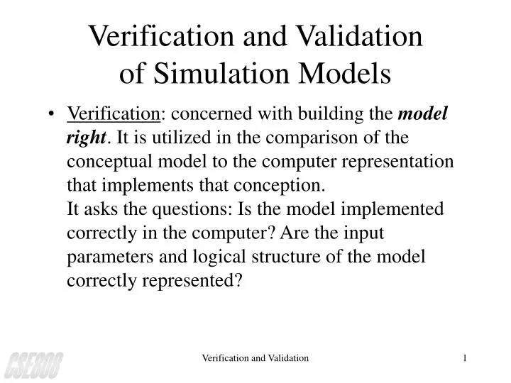
1. Verification and Validationof Simulation Models • Verification: concerned with building the model right. It is utilized in the comparison of the conceptual model to the computer representation that implements that conception. It asks the questions: Is the model implemented correctly in the computer? Are the input parameters and logical structure of the model correctly represented? Verification and Validation

2. Verification and Validationof Simulation Models (cont.) • Validation: concerned with building the right model. It is utilized to determine that a model is an accurate representation of the real system. Validation is usually achieved through the calibration of the model, an iterative process of comparing the model to actual system behavior and using the discrepancies between the two, and the insights gained, to improve the model. This process is repeated until model accuracy is judged to be acceptable. Verification and Validation

3. Verification of Simulation Models Many commonsense suggestions can be given for use in the verification process. 1. Have the code checked by someone other than the programmer. 2. Make a flow diagram which includes each logically possible action a system can take when an event occurs, and follow the model logic for each action for each event type. Verification and Validation

4. Verification of Simulation Models 3. Closely examine the model output for reasonableness under a variety of settings of the input parameters. Have the code print out a wide variety of output statistics. 4. Have the computerized model print the input parameters at the end of the simulation, to be sure that these parameter values have not been changed inadvertently. Verification and Validation

5. Verification of Simulation Models 5. Make the computer code as self-documenting as possible. Give a precise definition of every variable used, and a general description of the purpose of each major section of code. These suggestions are basically the same ones any programmer would follow when debugging a computer program. Verification and Validation

6. <Iterative process of calibrating a model> Calibration and Validationof Models Verification and Validation

7. Validation of Simulation Models As an aid in the validation process, Naylor and Finger formulated a three-step approach which has been widely followed: 1. Build a model that has high face validity. 2. Validate model assumptions. 3. Compare the model input-output transformations to corresponding input-output transformations for the real system. Verification and Validation

8. Validation of Model Assumptions • Structural involves questions of how the system operate (Example1) Data assumptions should be based on the collection of reliable data and correct statistical analysis of the data. Customers queueing and service facility in a bank (one line or many lines) 1. Interarrival times of customers during several 2-hour periods of peak loading (“rush-hour” traffic) Verification and Validation

9. Validation of Model Assumptions (cont.) 2. Interarrival times during a slack period 3. Service times for commercial accounts 4. Service times for personal accounts Verification and Validation

10. Validation of Model Assumptions (cont.) The analysis of input data from a random sample consists of three steps: 1. Identifying the appropriate probability distribution 2. Estimating the parameters of the hypothesized distribution 3. Validating the assumed statistical model by a goodness-of fit test, such as the chi-square or Kolmogorov-Smirnov test, and by graphical methods. Verification and Validation

11. Validating Input-Output Transformation (Example) : The Fifth National Bank of Jaspar The Fifth National Bank of Jaspar, as shown in the next slide, is planning to expand its drive-in service at the corner of Main Street. Currently, there is one drive-in window serviced by one teller. Only one or two transactions are allowed at the drive-in window, so, it was assumed that each service time was a random sample from some underlying population. Service times {Si, i = 1, 2, ... 90} and interarrival times {Ai, i = 1, 2, ... 90} Verification and Validation

12. Validating Input-Output Transformation (cont) Drive-in window at the Fifth National Bank. Verification and Validation

13. Validating Input-Output Transformation (cont) were collected for the 90 customers who arrived between 11:00 A.M. and 1:00 P.M. on a Friday. This time slot was selected for data collection after consultation with management and the teller because it was felt to be representative of a typical rush hour. Data analysis led to the conclusion that the arrival process could be modeled as a Poisson process with an arrival rate of 45 customers per hour; and that service times were approximately normally distributed with mean 1.1 minutes and Verification and Validation

14. Validating Input-Output Transformation (cont) standard deviation 0.2 minute. Thus, the model has two input variables: 1. Interarrival times, exponentially distributed (i.e. a Poisson arrival process) at rate l = 45 per hour. 2. Service times, assumed to be N(1.1, (0.2)2) Verification and Validation

15. Poisson arrivals Teller’s utilization M O D E L X11, X12,... rate = 45/hour Y1 = Random variables Service times X21, X22,... Average delay N(D2,0.22) Y2 One teller D1 = 1 Decision variables Mean service time “black box” Maximum line length D2 = 1.1 minutes Y3 One line D3 = 1 Input variables Output variables Model Validating Input-Output Transformation (cont) Model input-output transformation Verification and Validation

16. Validating Input-Output Transformation (cont) The uncontrollable input variables are denoted by X, the decision variables by D, and the output variables by Y. From the “black box” point of view, the model takes the inputs X and D and produces the outputs Y, namely (X, D) f Y or f(X, D) = Y Verification and Validation

17. Validating Input-Output Transformation (cont) Input Variables Model Output Variables, Y D = decision variables Variables of primary interest X = other variables to management (Y1, Y2, Y3) Poisson arrivals at rate Y1 = teller’s utilization = 45 / hour Y2 = average delay X11, X12,.... Y3 = maximum line length Input and Output variables for model of current bank operation (1) Verification and Validation

18. Validating Input-Output Transformation (cont) Input Variables Model Output Variables, Y Service times, N(D2,0.22) Other output variables of X21, X22,..... secondary interest Y4 = observed arrival rate D1 = 1 (one teller) Y5 = average service time D2 = 1.1 min Y6 = sample standard deviation (mean service time) of service times D3 = 1 (one line) Y7 = average length of line Input and Output variables for model of current bank operation (2) Verification and Validation

19. Validating Input-Output Transformation (cont) Statistical Terminology Modeling Terminology Associated Risk Type I : rejecting H0 Rejecting a valid model a when H0 is true Type II : failure to reject H0 Failure to reject an b when H0 is false invalid model (Table 1) Types of error in model validation Note: Type II error needs controlling increasing a will decrease b and vice versa, given a fixed sample size. Once a is set, the only way to decrease b is to increase the sample size. Verification and Validation

20. Validating Input-Output Transformation (cont) Y4 Y5 Y2 =avg delay Replication (Arrivals/Hours) (Minutes) (Minutes) 1 51 1.07 2.79 2 40 1.12 1.12 3 45.5 1.06 2.24 4 50.5 1.10 3.45 5 53 1.09 3.13 6 49 1.07 2.38 sample mean 2.51 standard deviation 0.82 (Table 2) Results of six replications of the First Bank Model Verification and Validation

21. Validating Input-Output Transformation (cont) Z2 = 4.3 minutes, the model responses, Y2. Formally, a statistical test of the null hypothesis H0 : E(Y2) = 4.3 minutes versus ----- (Eq 1) H1 : E(Y2) ¹ 4.3 minutes is conducted. If H0 is not rejected, then on the basis of this test there is no reason to consider the model invalid. If H0 is rejected, the current version of the model is rejected and the modeler is forced to seek ways to improve the model, as illustrated in Table 3. Verification and Validation

22. As formulated here, the appropriate statistical test is the t test, which is conducted in the following manner: Step 1. Choose a level of significance a and a sample size n. For the bank model, choose a = 0.05, n = 6 Step 2. Compute the sample mean Y2 and the sample standard deviation S over the n replications. Y2 = {1/n} Y2i = 2.51 minutes Validating Input-Output Transformation (cont) Verification and Validation

23. Validating Input-Output Transformation (cont) and S = {(Y2i - Y2)2 / (n - 1)}1/2 = 0.82 minute where Y2i, i = 1, .., 6, are shown in Table 2. Step 3. Get the critical value of t from Table A.4. For a two-sided test such as that in Equation 1, use ta/2, n-1; for a one-sided test, use ta, n-1 or -ta, n-1 as appropriate (n -1 is the degrees of freedom). From Table A.4, t0.025,5 = 2.571 for a two-sided test. Verification and Validation

24. Validating Input-Output Transformation (cont) Step 4. Compute the test statistic t0 = (Y2 - m0) / {S / Ön} ----- (Eq 2) where m0 is the specified value in the null hypothesis, H0 . Here m0 = 4.3 minutes, so that t0 = (2.51 - 4.3) / {0.82 / Ö6} = - 5.34 Step 5. For the two-sided test, if |t0| > ta/2, n-1 , reject H0 . Otherwise, do not reject H0. [For the one-sided test with H1: E(Y2) > m0, reject H0 if t > ta, n-1 ; with H1 : E(Y2) < m0 , reject H0 if t < -ta, n-1 ] Verification and Validation

25. Validating Input-Output Transformation (cont) Since | t |= 5.34 > t0.025,5 =2.571, reject H0 and conclude that the model is inadequate in its prediction of average customer delay. Recall that when testing hypotheses, rejection of the null hypothesis H0 is a strong conclusion, because P(H0 rejected | H0 is true) = a Verification and Validation

26. Validating Input-Output Transformation (cont) Y4 Y5 Y2 =avg delay Replication (Arrivals/Hours) (Minutes) (Minutes) 1 51 1.07 5.37 2 40 1.11 1.98 3 45.5 1.06 5.29 4 50.5 1.09 3.82 5 53 1.08 6.74 6 49 1.08 5.49 sample mean 4.78 standard deviation 1.66 (Table 3) Results of six replications of the REVISED Bank Model Verification and Validation

27. Validating Input-Output Transformation (cont) Step 1. Choose a = 0.05 and n = 6 (sample size). Step 2. Compute Y2 = 4.78 minutes, S = 1.66 minutes ----> (from Table 3) Step 3. From Table A.4, the critical value is t0.025,5 = 2.571. Step 4. Compute the test statistic t0 = (Y2 - m0) / {S / Ön} = 0.710. Step 5. Since | t |< t0.025,5 = 2.571, do not reject H0 , and thus tentatively accept the model as valid. Verification and Validation

28. Validating Input-Output Transformation (cont) To consider failure to reject H0 as a strong conclusion, the modeler would want b to be small. Now, b depends on the sample size n and on the true difference between E(Y2) and m0 = 4.3 minutes, that is, on d = | E(Y2) - m0 | / s where s , the population standard deviation of an individual Y2i , is estimated by S. Table A.9 and A.10 are typical operating characteristic (OC) curves, which are graphs of the probability of a Verification and Validation

29. Validating Input-Output Transformation (cont) Type II error b(d) versus d for given sample size n. Table A.9 is for a two-sided t test while Table A.10 is for a one-sided t test. Suppose that the modeler would like to reject H0 (model validity) with probability at least 0.90 if the true means delay of the model, E(Y2), differed from the average delay in the system, m0 = 4.3 minutes, by 1 minute. Then d is estimates by d = | E(Y2) - m0 | / S = 1 / 1.66 = 0.60 Verification and Validation

30. Validating Input-Output Transformation (cont) For the two-sided test with a = 0.05, use of Table A.9 results in b(d) = b(0.6) = 0.75 for n = 6 To guarantee that b(d) £0.10, as was desired by the modeler, Table A.9 reveals that a sample size of approximately n = 30 independent replications would be required. That is, for a sample size n = 6 and assuming that the population standard deviation is 1.66, the probability of accepting H0 (model validity) , when in fact the model is invalid Verification and Validation

31. Validating Input-Output Transformation (cont) (| E(Y2) - m0 | = 1 minute), is b = 0.75, which is quite high. If a 1-minute difference is critical, and if the modeler wants to control the risk of declaring the model valid when model predictions are as much as 1 minute off, a sample size of n = 30 replications is required to achieve a power of 0.9. If this sample size is too high, either a higher b risk (lower power), or a larger difference d, must be considered. Verification and Validation

32. Verification and Validation

33. Verification and Validation