Download
1 / 33
330 likes | 427 Views
This tutorial guides through constructing time series graphs, estimating autocorrelations, identifying trends, and fitting ARMA models for forecasting Swedish Consumer Price Index data. Graphical representations and statistical analyses are used to determine the most suitable model for accurate forecasts.

E N D
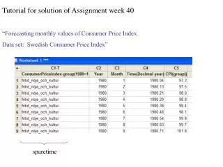
Tutorial for solution of Assignment week 40 “Forecasting monthly values of Consumer Price Index Data set: Swedish Consumer Price Index” sparetime
“Construct a time series graph for the monthly values of Consumer Price Index (Konsumentprisindex (KPI) in Swedish) for spare time occupation, amusement and culture (fritid, nöje och kultur in Swedish) (in file ‘sparetime.txt’).”
“Then estimate the autocorrelations and display them in a graph.” “Is there any obvious upward or downward trend?” Yes, upward, but turning at the end
“Are there any signs of long-time oscillations in the time series? No! Are there any signs of seasonal variation in the series?” Not visible!
“Do the autocorrelations cancel out quickly?” No! “Judge upon the need for differentiation according to ut = yt- yt-1 or vt = yt - yt-12 to get a time series that is suitable for forecasting with ARMA-models. Construct new graphs for the series obtained by differentiation and estimate the autocorrelations for these series.”
ut= yt – yt - 1 Not convincingly stationary! Diffuse pattern!
vt = yt – yt - 12 Definitely non-stationary!
“E.2. Fitting different ARMA-models Try different combinations of ARMA-models and differentiation to forecast the Consumer Price Index. Which model seems to give the best forecasts in this case.” From E.1.: Seems to be best to use first-order non-seasonal differences Chosen “design”: AR(1), AR(2) MA(1), MA(2) ARMA(1,1), ARMA(2,1), ARMA(1,2), ARMA(2,2)
Fixed to 1 in all models! Altered from model to model
AR(1): AR(2): Type Coef SE Coef T P AR 1 0.1170 0.0671 1.75 0.082 Constant 0.38522 0.04779 8.06 0.000 … MS = 0.512 DF = 222 Modified Box-Pierce (Ljung-Box) Chi-Squ Lag 12 24 36 48 … P-Value 0.000 0.000 0.000 0.000 Type Coef SE Coef T P AR 1 0.0770 0.0648 1.19 0.236 AR 2 0.3012 0.0655 4.60 0.000 Constant 0.27053 0.04576 5.91 0.000 … MS = 0.469 DF = 221 Modified Box-Pierce (Ljung-Box) Chi-Squ Lag 12 24 36 48 … P-Value 0.007 0.003 0.001 0.003 2 months forecasts: Forecast Lower Upper 195.472 194.070 196.875 195.925 193.823 198.027 2 months forecasts: Forecast Lower Upper 194.962 193.620 196.305 195.720 193.747 197.693
MA(1): MA(2): Type Coef SE Coef T P MA 1 -0.0741 0.0675 -1.10 0.273 Constant 0.43605 0.05146 8.47 0.000 … MS = 0.514 DF = 222 Modified Box-Pierce (Ljung-Box) Chi-Squ Lag 12 24 36 48 … P-Value 0.000 0.000 0.000 0.000 Type Coef SE Coef T P MA 1 -0.0592 0.0668 -0.89 0.376 MA 2 -0.2533 0.0670 -3.78 0.000 Constant 0.43664 0.06071 7.19 0.000 … MS = 0.479 DF = 221 Modified Box-Pierce (Ljung-Box) Chi-Squ Lag 12 24 36 48 … P-Value 0.000 0.000 0.000 0.000 2 months forecasts: Forecast Lower Upper 195.430 194.024 196.835 195.866 193.803 197.929 2 months forecasts: Forecast Lower Upper 195.146 193.789 196.503 196.032 194.056 198.009
ARMA(1,1): ARMA(2,1): * WARNING * Back forecasts not dying out rapidly Type Coef SE Coef T P AR 1 1.0186 0.0238 42.85 0.000 MA 1 0.9769 0.0006 1560.10 0.000 Constant -0.0117678 -0.0013602 8.65 0.000 … MS = 0.458 DF = 221 Modified Box-Pierce (Ljung-Box) Chi-Squ Lag 12 24 36 48 … P-Value 0.000 0.000 0.000 0.000 Type Coef SE Coef T P AR 1 0.3311 0.2045 1.62 0.107 AR 2 0.2711 0.0764 3.55 0.000 MA 1 0.2821 0.2129 1.33 0.186 Constant 0.17191 0.03287 5.23 0.000 … MS = 0.469 DF = 220 Modified Box-Pierce (Ljung-Box) Chi-Squ Lag 12 24 36 48 P-Value 0.004 0.001 0.000 0.001 2 months forecasts: Forecast Lower Upper 194.516 193.190 195.843 194.114 192.199 196.029 2 months forecasts: Forecast Lower Upper 194.746 193.403 196.088 195.300 193.355 197.246
ARMA(1,2): ARMA(2,2): Type Coef SE Coef T P AR 1 0.6136 0.1635 3.75 0.000 MA 1 0.5577 0.1679 3.32 0.001 MA 2 -0.2202 0.0763 -2.89 0.004 Constant 0.16753 0.03043 5.51 0.000 … MS = 0.472 DF = 220 Modified Box-Pierce (Ljung-Box) Chi-Squ Lag 12 24 36 48 … P-Value 0.002 0.001 0.000 0.000 * ERROR * Model cannot be estimated with these data. 2 months forecasts: Forecast Lower Upper 194.728 193.382 196.075 195.214 193.256 197.173
None of the models are satisfactory in goodness-of-fit and prediction intervals are quite similar (slightly more narrow for the more complex models). Maybe second-order non-seasonal differences would work? wt = ut– ut – 1 =(yt – yt – 1) – (yt – 1 – yt – 2) = yt – 2yt – 1 + yt – 2
How about first order seasonal differences on the first-order non-seasonal differences? zt= ut– ut – 12 = (yt – yt – 1)– (yt – 12 – yt – 13)
Tricky to identify the correct model. Clearly a seasonal model must be used, most probably with at least one MA –term Non-seasonal part more difficult. ARMA(1,1) ?
Type Coef SE Coef T P AR 1 -0.6368 1.2524 -0.51 0.612 MA 1 -0.6085 1.2902 -0.47 0.638 SMA 12 0.8961 0.0484 18.51 0.000 Constant -0.07528 0.01129 -6.67 0.000 Differencing: 1 regular, 1 seasonal of order 12 Number of observations: Original series 225, after differencing 212 Residuals: SS = 77.9325 (backforecasts excluded) MS = 0.3747 DF = 208 Modified Box-Pierce (Ljung-Box) Chi-Square statistic Lag 12 24 36 48 Chi-Square 12.9 22.8 28.9 36.0 DF 8 20 32 44 P-Value 0.115 0.300 0.626 0.800 2 months forecasts: Forecast Lower Upper 194.971 193.771 196.171 195.580 193.907 197.253
Compare with ARIMA(0,1,0,0,1,1)12 Type Coef SE Coef T P SMA 12 0.9039 0.0472 19.15 0.000 Constant -0.045964 0.006893 -6.67 0.000 Differencing: 1 regular, 1 seasonal of order 12 Number of observations: Original series 225, after differencing 212 Residuals: SS = 78.0539 (backforecasts excluded) MS = 0.3717 DF = 210 Modified Box-Pierce (Ljung-Box) Chi-Square statistic Lag 12 24 36 48 Chi-Square 12.5 21.8 28.0 34.8 DF 10 22 34 46 P-Value 0.254 0.475 0.757 0.887 Slightly smaller MS! 2 months forecasts: Forecast Lower Upper 194.987 193.792 196.182 195.587 193.897 197.277
“E.3. Residual analysis Construct a graph for the residuals (the one-step-ahead prediction errors) and examine visually if there is any pattern in the residuals indicating that the selected forecasting model is not optimal.” Residual plots for ARIMA(1,1,1,0,0,0) ARIMA(1,1,1,0,1,1)12 ARIMA(0,1,0,0,1,1)12
ARIMA(1,1,1,0,0,0): Non-satisfactory
ARIMA(1,1,1,0,1,1)12 Satisfactory!
ARIMA(0,1,0,0,1,1)12 Satisfactory!
“F. ARMA-models and exponential smoothing Data set: The Dollar-Danish Crowns Exchange rates Consider the time series of monthly exchange rates US$/DKK.”
“At first, calculate forecasts by using exponential smoothing and note the prediction formula.” Change scale so that y-axis starts at 0 (and ends at 10) Single exponential smoothing will probably work well. Optimize
Calculate forecasts for 6 months (an arbitrarily chosen value)
Forecasts Period Forecast Lower Upper 96 6.31118 5.94410 6.67825 97 6.31118 5.94410 6.67825 98 6.31118 5.94410 6.67825 99 6.31118 5.94410 6.67825 100 6.31118 5.94410 6.67825 101 6.31118 5.94410 6.67825 Prediction formula:
“Then calculate forecasts by fitting a MA(1)-model to first differences of the original series (i.e. you must differentiate the series once).”
Final Estimates of Parameters Type Coef SE Coef MA 1 0.0052 0.1043 Constant 0.00537 0.02027 Forecasts from period 95 95 Percent Limits Period Forecast Lower Upper 96 6.31652 5.92916 6.70387 97 6.32189 5.77550 6.86828 98 6.32726 5.65864 6.99587 99 6.33263 5.56091 7.10434 100 6.33800 5.47542 7.20057 101 6.34336 5.39862 7.28811 “How does the prediction formula look like in this case?”
“How do the forecasts differ between the two different methods of forecasting?” SES ARIMA(0,1,1) Forecasts from period 95 95 Percent Limits Period Forecast Lower Upper 96 6.31652 5.92916 6.70387 97 6.32189 5.77550 6.86828 98 6.32726 5.65864 6.99587 99 6.33263 5.56091 7.10434 100 6.33800 5.47542 7.20057 101 6.34336 5.39862 7.28811 Forecasts Period Forecast Lower Upper 96 6.31118 5.94410 6.67825 97 6.31118 5.94410 6.67825 98 6.31118 5.94410 6.67825 99 6.31118 5.94410 6.67825 100 6.31118 5.94410 6.67825 101 6.31118 5.94410 6.67825