Planning with Local Search
520 likes | 683 Views
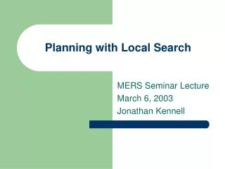
Planning with Local Search. MERS Seminar Lecture March 6, 2003 Jonathan Kennell. Presentation Outline. Planning Overview What is planning? – 5 mins. Taxonomy of planners – 40 mins. (or everything you ever wanted to know about planning in approximately 40 minutes) 5 minute break LPG

Planning with Local Search
E N D
Presentation Transcript
Planning with Local Search MERS Seminar Lecture March 6, 2003 Jonathan Kennell
Presentation Outline • Planning Overview • What is planning? – 5 mins. • Taxonomy of planners – 40 mins.(or everything you ever wanted to know about planning in approximately 40 minutes) 5 minute break • LPG • Background information (WalkSAT) – 10 mins. • Linear action graphs and precedence graphs – 10 mins. • WalkPlan planning algorithm – 10 mins. • Example – 10 mins.
What is Planning? • Input • Set of world-states • Action operators (fn: world-state world-state) • Initial world-state • Goal (possibly a partial state / set of world-states) • Output • Ordering of actions From 6.834J POP lecture
World State • Set of facts and their degree of truth • Examples: • (Student Jonathan) // true • (Likes Jonathan Golf) // false • (Graduating Jonathan June) // unknown * • Note: lisp notation used extensively in planning community • * Most planners don’t consider unknown facts
Planning Operators • Fn: world-state world-state • Generally use STRIPS format: • Preconditions: facts that must be true before action can occur • Effects: facts that become true (or false) after the action occurs • Extra properties: • Separate start / invariant / end conditions and effects • Durations • Resource constraints (:action Move (:params ((robot ?r) (location ?a) (location ?b)) (:preconds (at ?r ?a)) (:effects (and (not (at ?r ?a)) (at ?r ?b))))
Mutual Exclusion • Sometimes planning operators conflict with each other – we call a pair of conflicting operators mutex • Examples of mutex actions: • Interference: A deletes precondition or effect of B • Competing Needs: A and B have mutex preconditions • Planner must ensure no mutex actions co-occur.
Activity-A Activity-C fact-L fact-J fact-O fact-M Start End Activity-B Activity-D fact-K fact-P fact-N What is a plan? • A plan is an ordering of actions that will transition the system from the initial state to the goal state.
Completeness / Consistency / Minimality • Complete Plan • A plan is complete IFF every precondition of every activity is achieved. • An activity’s precondition is achieved IFF: • The precondition is the effect of a preceding activity (support), and • No intervening step conflicts with the precondition (mutex). • Consistent Plan • The plan is consistent IFF the temporal constraints of its activities are consistent (the associated distance graph has no negative cycles), and • no conflicting (mutex) activities can co-occur. • Minimal Plan • The plan is minimal IFF every constraint serves a purpose, i.e., • If we remove any temporal or symbolic constraint from a minimal plan,the new plan is not equivalent to the original plan
Variations on Classical Planning • Temporal planning • Actions have durations • Planning with resources • Facts can be quantified • Planning with uncertainty • Effects / durations of actions not guaranteed
SHOP2 Macro Decomposition (restricted plan-space) Kirk TPN Planner TLPlan Global Search Forward Chaining / Backward Propagation (entire plan-space) Kirk Deductive Controller Local Search LPG Graphplan Plan Graph (condensed plan-space) LPGP Taxonomy of Planners Planners
Forward Chaining / Backward Propagation • Searches through entire plan-space by non-deterministically adding actions to plan candidates. • Advantages: • generative (does not require strategies) • expressive (can handle time, resources, easily) • Disadvantages: • Inherently slow (plan-space is enormous)
Etc. Forward Chaining Example Familiar tradeoff: Efficient pruning methods versus optimality.
Case Study: TLPlan • TLPlan (Temporal Logic Planner) by Fahiem Bacchus and Froduald Kabanza • TLPlan is based on a forward-chaining planner • TLPlan uses domain-dependent temporal logic to prune the search space
TLPlan: First-order Temporal Logic • Definition:First-order linear temporal logic • standard first-order logic, plus: • U (until), □ (always), ◊ (eventually), ○ (next) • Boundedquantifiers: • [x:y]x . y(x)(x) • [x:y] x . y(x)(x) • Example: • □(on(B,C) (on(B,C) U on(A,B))) • Asserts that whenever we enter a state in which B is on C it remains on C until A is on B
TLPlan: Formula Progression Algorihtm • The Progress algorithm is used to check control strategies as the system searches for a plan. • Inputs: An LTL formula f and a world w (generated by forward-chaining) • Output: A new formula f+, also expressed as an LTL formula, representing the progression of f through the world w. • Algorithm:Progress(f,w) • Case • f = is atomic: if w entails f, f+ := TRUE, else f+ = FALSE • f = f1 f2: f+ := Progress(f1,w) Progress(f2,w) • f = f1: f+ := Progress(f1,w) • … etc. … (see paper for complete algorithm)
TLPlan Example Forward chaining begins… Rules: Etc. (Any color) This thread is efficiently guided by the rules This thread is not guided well since no rules apply.This results in pure forward-chaining search.
TLPlan Review • TLPlan has been around in various implementations since 1995, although improvements have been made as recently as last year. • TLPlan functions initially as a forward-chaining planner, but can use logical rules to guide its search and prune unfeasible threads. • TLPlan was the fastest domain-specific planner in the 2002 AIPS competition.
Domain Knowledge • Planning is hard – the most general planners are extremely slow • To increase speed, some planners sacrifice generality by using domain-specific strategies. • TLPlan encodes the strategy into the goal specification, while other planners decouple the goals and the strategies.
Forward Chaining Speedup • Many researches have focused on discovering ways to help speedup domain-independent forward chaining planners. • Ex. SAPA by Minh B. Do & Subbarao Kambhampati • Methods focus on estimating plan cost using: • Relaxed plan-graphs • Estimated remaining cost to goal • Cost metrics • Ex. # actions, plan duration, etc.
SHOP2 Macro Decomposition (restricted plan-space) Kirk TPN Planner TLPlan Global Search Forward Chaining / Backward Propagation (entire plan-space) Kirk Deductive Controller Local Search LPG Graphplan Plan Graph (condensed plan-space) LPGP Taxonomy of Planners Planners
Plan Graph • Plan-graph based planners first construct a compact representation of the plan-space (the plan-graph), and then search that space. • Plan-graphs contains all possible plans up to a certain size, excluding incomplete plans with co-occurring binary mutex actions. • Plan-graphs do not exclude all invalid plans, and depending on the domain may yield extremely efficient or inefficient results. • Advantages: • generative • much faster than most forward-chaining planners • plan-graph can be generated in polynomial time and space • Disadvantages: • plan-graphs are less expressive (resources and time difficult) • in certain domains, search of plan-graph can be very inefficient
Forward Chaining vs. Plan Graph Forward Chaining Plan Graph
Case Study: Graphplan Note the compact structure in this graph – it’s polynomial in size!
Case Study: LPGP • Idea: • use Graphplan to identify complete plan (action structure) • then use Linear Programming to determine plan consistency and perform scheduling (assign durations to actions) • Advantage: • Two-phase approach accomplishes temporal planning with the speed of a plan-graph based planner • Disadvantages: • Cannot optimize over time (only optimizes over makespan) • Two-phase approach is potentially very inefficient • no temporal conflicts are used to guide Graphplan search • search not incremental – LP must be started from scratch each time
SHOP2 Macro Decomposition (restricted plan-space) Kirk TPN Planner TLPlan Global Search Forward Chaining / Backward Propagation (entire plan-space) Kirk Deductive Controller Local Search LPG Graphplan Plan Graph (condensed plan-space) LPGP Taxonomy of Planners Planners
Macro Decomposition • Operates similar to context-free grammar • planner non-deterministically expands “macro-activities” until all plan actions are primitive. • rules ensure that planner only explores space of complete plans • Planner still must ensure plan consistency. • Advantages • Fast • Disadvantages • all achieving strategies must be pre-encoded into macros • non-optimal: explores restricted plan-space, potentially excluding optimal solutions
Case Study: SHOP2 • SHOP2 by Dana Nau, Hector Munoz-Avila, Yue Cao, Amnon Lotem and Steven Mitchell • SHOP2 works similar to the task-decomposition mechanism in Kirk • SHOP2 problems consist of: • Operators (with preconditions, add-effects and delete-effects) • Methods (rules for how to progress the plan) • Initial conditions and goals • SHOP2 is fairly fast, but all plan happenings must be pre-designed (at some level) by a programmer. • SHOP2 plans do not support concurrency
SHOP2 Example (defdomain basic-example ( (:operator (pickup ?a) () () ((have ?a))) (:operator (drop ?a) ((have ?a)) ((have ?a)) ()) (:method (swap ?x ?y) ((have ?x)) ((drop ?x) (pickup ?y)) ((have ?y)) ((drop ?y) (pickup ?x))))) (defproblem problem1 basic-example ((have banjo)) ((swap banjo kiwi))) Preconds Delete-effects Add-effects Condition Strategy Allows one method todecompose into multiplepossible subplans, dependingon the current state Initial Condition Start Strategy
SHOP2 In Action (defdomain basic-example ( (:operator (pickup ?a) () () ((have ?a))) (:operator (drop ?a) ((have ?a)) ((have ?a)) ()) (:method (swap ?x ?y) ((have ?x)) ((drop ?x) (pickup ?y)) ((have ?y)) ((drop ?y) (pickup ?x))))) (defproblem problem1 basic-example ((have banjo)) ((swap banjo kiwi))) (defdomain basic-example ( (:operator (pickup ?a) () () ((have ?a))) (:operator (drop ?a) ((have ?a)) ((have ?a)) ()) (:method (swap banjo kiwi) ((have banjo)) ((drop banjo) (pickup kiwi)) ((have kiwi)) ((drop kiwi) (pickup banjo))))) (defproblem problem1 basic-example ((have banjo)) ((swap banjo kiwi))) State: (have kiwi) ? (have banjo) DONE
Case Study: Kirk TPN Planner Macro-Activity() [l,u] Decomposition 1 Decomposition 2
Presentation Outline • Planning Overview • What is planning? – 5 mins. • Taxonomy of planners – 40 mins.(or everything you ever wanted to know about planning in approximately 40 minutes) 5 minute break • LPG • Background information (WalkSAT) – 10 mins. • Linear action graphs and precedence graphs – 10 mins. • WalkPlan planning algorithm – 10 mins. • Example – 10 mins.
SHOP2 Macro Decomposition (restricted plan-space) Kirk TPN Planner TLPlan Global Search Forward Chaining / Backward Propagation (entire plan-space) Kirk Deductive Controller Local Search LPG Graphplan Plan Graph (condensed plan-space) LPGP Taxonomy of Planners Planners
Local Search: WalkSAT • WalkSAT is a randomized algorithm for solving SAT (propositional satisfiability) problems. • It builds on the DPLL algorithm, but utilizes local search and randomness.
WalkSAT • Problem: • Find a satisfying assignment to a logic formula • (A || !B) && (B || !C) && (C || !A) && (A || B || C) • WalkSAT: • Pick a random assignment to the variables • Until formula satisfied (or up to some max # of iterations), • Choose an unsatisfied clause and enumerate the ways of adjusting the variables in order to satisfy it • With probability p • Choose the best-utility adjustment • Else • Choose a random adjustment
WalkSAT Example • (A || !B) && (B || !C) && (C || !A) && (A || B || C) • Pick !A, !B, !C • (A || !B) && (B || !C) && (C || !A) && (A || B || C) • Options are to switch A, B, or C • Pick A, !B, !C • (A || !B) && (B || !C) && (C || !A) && (A || B || C) • Options are to switch A or C • Pick A, !B, C • (A || !B) && (B || !C) && (C || !A) && (A || B || C) • Options are to switch B or C • Pick A, B, C • (A || !B) && (B || !C) && (C || !A) && (A || B || C) • Formula Satisfied!
WalkSAT Discussion • WalkSAT has proven to be very fast at solving complicated SAT problems • WalkSAT can solve some problems that systematic algorithms simply can’t handle • Due to randomness, WalkSAT is incomplete • WalkSAT may fail to discover a solution
Introduction to LPG • LPG (local search for plan-graphs) – by Alfonso Gerevini and Ivan Serina • Blackbox mapped the planning problem to a CSP and solved it using a SAT solver. • LPG unifies the planning and WalkSAT algorithms to create the WalkPlan search algorithm.
LPG Big Idea • Big Idea: • Start with a random plan • While plan is incorrect / inconsistent • Identify and repair conflict • Basically the same idea of WalkSAT, but applied to a special form of plan-graph
Temporal Action Graphs • Definitions: • Action-graph: the subset of a plan-graph containing the action layers • Support: a fact is said to be “supported” if it is achieved by some action in the previous action layer • Conflict: • a mutex between two actions • an action with an unsupported precondition
Linearization of Action Graphs • An Action Graph can be made linear by allowing only one action per action layer. • The layers no longer explicitly represent an ordering of time (temporal concurrency is still possible) • The layer ordering simply presents an action sequence for the purposes of establishing fact support relationships.
A0 No-op No-op No-op A0 A1 A2 Example: Linear Action Graph A B C A B C A B C A B C A B C A plan-graph consists of alternating fact layers and action layers. The actions alone constitute an action graph. LPG operates directly on the action graph structure, inserting and removingactions from various action layers as it repairs incomplete plans.
Conflicts and Repair • An incomplete plan is manifested as an action graph with conflicts. • Example conflicts with resolution (repair) strategies:
LPG’s WalkPlan Planning Algorithm LPG Algorithm Generate Initial Plan • LPG: • Generate an initial dummy plan, P, either… • Randomly • By adding actions to support all facts ignoring mutexes, or • Via some front-end plan generator • Randomly choose a conflict in the action-graph, C • Identify all possible ways of resolving C and evaluate them using the action evaluation function • Resolution techniques include: removing one of two mutex actions, adding a supporting action for an unsupported fact, or removing an action that has an unsupported precondition • If a conflict resolution has cost 0, the plan is complete • Note: The action evaluation function uses Lagrange multipliers to dynamically weight the different factors in the action evaluation function • If a resolution introduces no new conflicts, apply it and go to step (2)Else, • with probability p, randomly choose a resolution, apply it and go to step (2) • with probability 1-p, choose the lowest cost conflict resolution, apply it and go to step (2) • Note: The resolution step includes a mechanism for extending the plan-graph Choose Conflict Resolve & Evaluate Resolution Selection
A0 No-op No-op No-op No-op No-op No-op A0 A1 A1 B A2 A2 C C LPG Example A B C A B C A B C A B C A B C Permanently mutex actionsin the same action layer(resolved by removing one of the two actions) Unsupported precondition(resolved by adding achievingaction at previous action layer) Unsupported precondition(resolved by removing theconflicting action) Unsupported precondition(resolved by adding achievingaction at previous action layer) Note: No-ops are propagated during conflict resolution Initial Conditions: ( nil ) Goals: ( A, B, C ) Actions: A0: preconds ( nil ) effects ( A ) A1: preconds ( A ) effects ( A, B ) A2: preconds ( A, B ) effects ( C ) Initial dummy plan Identify conflict Resolve conflict Plan complete
LPG Analysis • Advantages: • LPG is fast – four orders of magnitude faster than the leading optimal planners • LPG is domain-independent • LPG can easily handle resources and durative actions • Disadvantages: • LPG is randomized, so plans are not usually optimal and often contain extraneous actions • LPG includes option to continue searching for multiple solutions, in the hope of finding better plans • While maintaining expressivity, LPG sacrifices optimality for speed.