Download
1 / 11
110 likes | 216 Views
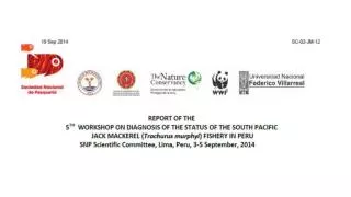
Relationships between the main characteristics of the environment and the JM distribution. Catches , abundance and biomass 3. Geostatistica abundance stimation ( A) Regionalización de las calas, y cálculo de la Inercia (I) y Centro de Gravedad (CG).

E N D
Relationships between the main characteristics of the environment and the JM distribution
Geostatisticaabundancestimation (A) Regionalización de las calas, y cálculo de la Inercia (I) y Centro de Gravedad (CG) • Estimación de la Abundancia (A) en base a captura media por región (quincenas) como indicador de la densidad (Q, t/mn2). • Estimación de indicador de Esfuerzo (E) en base al númer de calas (NCi) y número efectivo de meses de pesca (M):
TSM 15° a 26°C SSM 35.05 a 35.15 UPS Batimetría >150m Clorofila 0.3 a 5 ug.L-1 Anomalías -1 a +1 Térmicas • Hábitat Potencial de Jurel • Construido como el promedio de probabilidades (0 a 1) según 6 variables que mejor representan el hábitat potencial del jurel. • Temperatura, anomalías térmicas, salinidad, clorofila, profundidad, y distancia a la costa para cuadros de 26 mn2 c/u con P > 0. • Determina el área total probable de distribución de jurel (hábitat potencial).
Conclusions • The year 2013 began as a cold year, but strong anomalies occurred from June to August (-1.4ºC), during whichthree Kelvin waves arrived in the Peruvian waters in autumn, 2014, resulting in an increase of the SST (+3.5ºC). • In September the SST is still above the average of this month (+0.1 to +0.3ºC). Using these hydrologic results, the potential habitat of jack mackerel could be evaluated and appeared to be less extended than in 2011, especially in the north. Besides, it has been demonstrated that the depth of the oxycline is a key parameter for drawing the potential habitat, which will be done in the future workshops. • The demographic structure of the population was analyzed and showed that during the 1st trimester 2014 the bulk of the catch was done on 3-year old fish. The growth curve of the stock in Peruvian waters is significantly different from the one in other areas of the fish distribution, confirming the specificity of the Peruvian (Far North) subpopulation. • Except in 2011, the fishing season in 2012-2014 was mostly limited to the period January-May (summerautumn). Nevertheless, compared to the former years, 2014 presented warm situations (Kelvin waves), which effect is to concentrate jack mackerel closer to the coast, making it more accessible to the fishery. The CPUE is the lowest in 2014 compared to the high values of 2011-2012 (normal to warm situation) and the medium values of 2013 (colder situation), which is likely due to the extension of the fishing ground at larger distance to the coast. The biomass measured with acoustics varied between 20 000 and 332 000 tons. During the 4 years monitored, the biomass fluctuated between 8 000 (March, 2013) and 758 000 tons (February, 2011). The distribution area fluctuated between 268 MN2 (May, 2013) and 3 373 NM2 (June 2011); and the catch between 1 200 and 73 000 tons. The total catch for the 4 years was 518 000 tons.