Download
1 / 19
200 likes | 356 Views
Comparing a series of unsupervised c lassifications ran on a Landsat-5 image of the Salton Sea . Nicole Stotz Geog 342 Spring 2010. Project Summary Compare increasing numbers of unsupervised classes, and the affect on image output using a Landsat-5 image of the Salton Sea.

E N D
Comparing a series of unsupervised classifications ran on a Landsat-5 image of the Salton Sea Nicole Stotz Geog 342 Spring 2010
Project Summary • Compare increasing numbers of unsupervised classes, and the affect on image output using a Landsat-5 image of the Salton Sea. • Part 1: Ran a series of unsupervised classifications, starting with 6 classes and ending with 30. Compared transformed divergence reports for each classification. • Part 2: Land cover classification – used the recode tool on a series of unsupervised classifications, comparing how the number of signatures affect a simplified landcover scheme with 5 classes.
Acquiring An Image • Study area: Salton Sea/Imperial County, CA • glovis.usgs.gov for Landsat imagery • Originally I downloaded a Landsat 7 image – post 2003 images have striping because of damage to the satellite’s scan-line corrector. I didn’t know how to correct this, so I chose the same view from Landsat 5. Striping in Landsat 7 image
Salton Sea, Landsat-5 image acquired Feb. 16, 2010 • 28.5-meter data. • 7 bands, coverage area of 183 x 170 km. • Image file included individual .tif for each band. • Band files were converted from .tif to .img files, and then stacked into a single layer using ERDAS.
Part 1: Comparing unsupervised classifications • 6 classes as a starting point – a smaller number wouldn’t work with the spectral diversity of the image. • 30 classes as an end point – a balance of demonstrating a trend, and data overload. • 14 unsupervised classifications ran, 15 iterations per classification. • Collected transformed divergence reports and dendrograms for each unsupervised classification.
Output examples…. 7 classes vs. 30 classes (Lots of other intermediary classes not shown)
Transformed divergence tests were ran on every unsupervised classification. What sort of patterns emerged? -The class confusion threshold is 1800, with 2000 meaning perfect seperability. -Initial transformed divergence tests ran on unsupervised classifications of 6, 7, and 8 classes revealed a trend in class seperability. -As more classes are specified for an unsupervised classification, class confusion does increase, but it is a finer grained spectral confusion.
7 class unsupervised classification, colored to show class confusion • 4:5(1645), 3:4(1561), 5:6(1655), 6:7(1620) – classes that are spectrally confused. • Desert areas (dunes, barren, shrub) are difficult to tell from urban areas (yellow, brown, orange, grey). • Green areas represent both crops and woodland.
14 class unsupervised classification, colored to show class confusion Crops and woodland are now separate, but there is still much confusion between urban areas and rocky desert hills (orange, pink, blue, purple, etc).
Dendrogram for 14 class unsupervised classification. Classes in the center are spectrally confused desert and urban areas.
Conclusions from Part 1: • Increasing classes in an unsupervised classification allows for greater class seperability. • Comparing signature statistics along with transformed divergence tests can help identify trends that may be passed over in a visual inspection. • Mixed pixel areas lead to the greatest class confusion. Especially noticeable in the belt of irrigated desert cropland between the Salton Sea and Mexicali. • Did not anticipate that urban areas would share spectral characteristics of desert shrub land and rocky hills.
Part Two: Landcover classification • Increasing classes in an unsupervised classification affects class seperability: how does this factor into a simple landcover scheme of 5 classes? • Used the recode tool on unsupervised classifications to create 10 landcover images. • Planned to increasethe signatures per class by 1 for each image: image 1 (6 signatures) , image 2 (12 signatures)…image 10 (60 signatures). • Started with a 6 class scheme based on a CalFire landcover overlay: cropland, water, urban, woodland/grassland, desert, barren. • Realized my image wasn’t detailed enough to pick out barren areas. Desert became a catch-all category, and I used a 5 class scheme: cropland, water, urban, woodland/grassland, desert. • Not sure how much this affected my results, but the general trend I saw is still useful.
CalFire landcover overlay, clipped to extent of Landsat scene. • 13 landcover classes represented. • The overlay stops at the border. Since the Landsat scene extends only a few miles into Mexico, I assumed that the terrain is close enough to that of the California overlay that I could still use it as for general comparison.
Sample output… 12 classes recoded vs 60 classes recoded
Comparison of 12 vs 60 classes recoded • Final output for the 12 class recode • 1Ag – 1-2 • 2Water- 3 • 3Trees/grassland – 6 • 4Urban- none • 5Desert - 4-5, 7-12 • *6Other - 1 (not shown) • *6Other = bands only on the edge of the image • Final output for the 60 class recode • 1Ag –6-9, 11 • 2Water - 2 • 3Trees/grassland- 4, 12, 15, 22 • 4Urban - 24 • 5Desert- 13, 14, 16-21, 23, 25-46, 48-60 • *6Other - 3, 5, 10, 47 (not shown) The most signatures ended up in the Desert class, the fewest in the Urban class, in all 10 image recodes.
12 class recode vs 60 class recode Used the swipe tool in ERDAS to compare the Urban class in my scheme. Left = 60 class recode Right = 12 class recode Black speckled area is about the location of El Centro – it appears as desert in the 12 class recode on the right. The Urban class was the hardest to define. Even though El Centro did not appear in the 12 class recode image, it’s possible to define its boundaries by the missing area in the middle of the cropland.
Another comparison… Left = 60 class recode Right = 12 class recode Green area represents Trees/grassland class. This is a range of mountains between the Imperial Valley and San Diego. More signatures assigned to this class in the 60 class recode more accurately represent the actual vegetation.
CalFire 13 class landcover layer as a 75% transparent overlay on the 60 class recode image.
Conclusions from Part 2: • Signature classification didn’t go as planned during the recode. Some classes had more or less signatures assigned than planned for. • More signatures assigned to a class increases the accuracy of the classification. • Assigning signatures for the Urban class was difficult, leading to inaccuracies in the landcover images. • Next time, use higher number of classes in an unsupervised classification if it’s a basis for landcover classification. • A higher resolution image would have made classifications more accurate. • Using recode on an unsupervised classification is a good way to create a basic landcover classification, but the inaccuracies make it suitable for basic analysis only.