Download
1 / 30
300 likes | 441 Views
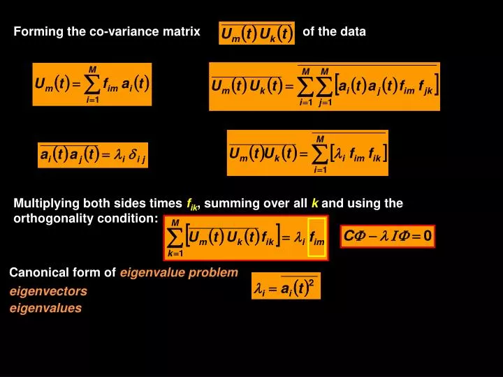
Forming the co-variance matrix. of the data. Multiplying both sides times f ik , summing over all k and using the orthogonality condition:. Canonical form of eigenvalue problem. eigenvectors. eigenvalues. I is the unit matrix and are the EOFs.

E N D
Forming the co-variance matrix of the data Multiplying both sides times fik, summing over all k and using the orthogonality condition: Canonical form of eigenvalue problem eigenvectors eigenvalues
I is the unit matrix and are the EOFs Eigenvalue problemcorresponding to a linear system:
Matrix = [6637,18] rows > columns
Matrix ul = [6637,18] >> uc=cov(ul); >> u1=ul(:,1); >> sum((u1-mean(u1)).^2)/(length(u1)-1) ans = 9.6143 >> u2=ul(:,2); >> sum((u1-mean(u1)).*(u2-mean(u2)))/(length(u1)-1) ans = 10.1154
Covariance Matrix Maximum covariance at surface
>> uc=cov(ul); >> [v,d]=eig(uc); eigenvalues (or lambda) >> lambda=diag(d)/sum(diag(d));
>> uc=cov(ul); >> [v,d]=eig(uc);
>> uc=cov(ul); >> [v,d]=eig(uc); >> v=fliplr(v);
Mode 2 13.2% Mode 1 85.3%
>> ts=ul*v; ts=[6637,18] Mode 1 85.3% Mode 2 13.2% Mode 2 13.2% Mode 1 85.3%
>>for k=1:nz vt(k,:,:)=ts(:,k)*v(:,k)'; end vt=[18, 6637,18] mode # evolution in time time series # >> v1=squeeze(vt(1,:,:))’; >> v2=squeeze(vt(2,:,:))’; Depth (m)
Complex Empirical Orthogonal Functions – James River Data u v Linear combination of spatial predictors or modes that are normal or orthogonal to each other
Rotated 49 degrees Streamwise Cross-stream
Mode 1 96.5% Mode 1
Mode 2 2.5% Mode 2
Streamwise Mode 1 96.5% cross-stream
Mode 1 96.5% Principal-axis Mode scaling cross-axis
Mode 2 2.5% Streamwise Mode scaling Cross-stream
Mode 2 2.5% Streamwise Mode scaling cross-stream
Mode 1 75% m/s m/s m/s
Mode 2 22% m/s m/s m/s
Phase of EOFS Mode 2 Depth (m) Mode 1 radians
streamwise cross-stream
streamwise cross-stream