Clustering & Memory-Based Reasoning
Learn about clustering in data mining, distance/similarity measures, vector representation, common algorithms, and clustering examples.

Clustering & Memory-Based Reasoning
E N D
Presentation Transcript
Clustering&Memory-Based Reasoning Bamshad Mobasher DePaul University
What is Clustering in Data Mining? • Cluster: • a collection of data objects that are “similar” to one another and thus can be treated collectively as one group • but as a collection, they are sufficiently different from other groups • Clustering • unsupervised classification • no predefined classes Clustering is a process of partitioning a set of data (or objects) in a set of meaningful sub-classes, called clusters Helps users understand the natural grouping or structure in a data set
Distance or Similarity Measures • Measuring Distance • In order to group similar items, we need a way to measure the distance between objects (e.g., records) • Note: distance = inverse of similarity • Often based on the representation of objects as “feature vectors” Term Frequencies for Documents An Employee DB Which objects are more similar?
Distance or Similarity Measures • Properties of Distance Measures: • for all objects A and B, dist(A, B) ³ 0, and dist(A, B) = dist(B, A) • for any object A, dist(A, A) = 0 • dist(A, C) £ dist(A, B) + dist (B, C) • Representation of objects as vectors: • Each data object (item) can be viewed as an n-dimensional vector, where the dimensions are the attributes (features) in the data • Example (employee DB): Emp. ID 2 = <M, 51, 64000> • Example (Documents): DOC2 = <3, 1, 4, 3, 1, 2> • The vector representation allows us to compute distance or similarity between pairs of items using standard vector operations, e.g., • Dot product • Cosine of the angle between vectors • Euclidean distance
Distance or Similarity Measures • Common Distance Measures: • Manhattan distance: • Euclidean distance: • Cosine similarity:
Distance (Similarity) Matrix • Similarity (Distance) Matrix • based on the distance or similarity measure we can construct a symmetric matrix of distance (or similarity values) • (i, j) entry in the matrix is the distance (similarity) between items i and j Note that dij = dji (i.e., the matrix is symmetric. So, we only need the lower triangle part of the matrix. The diagonal is all 1’s (similarity) or all 0’s (distance)
Example: Term Similarities in Documents • Suppose we want to cluster terms that appear in a collection of documents with different frequencies • We need to compute a term-term similarity matrix • For simplicity we use the dot product as similarity measure (note that this is the non-normalized version of cosine similarity) • Example: Each term can be viewed as a vector of term frequencies (weights) N = total number of dimensions (in this case documents) wik = weight of term i in document k. Sim(T1,T2) = <0,3,3,0,2> * <4,1,0,1,2> 0x4 + 3x1 + 3x0 + 0x1 + 2x2 = 7
Example: Term Similarities in Documents Term-Term Similarity Matrix
Similarity (Distance) Thresholds • A similarity (distance) threshold may be used to mark pairs that are “sufficiently” similar Using a threshold value of 10 in the previous example
T3 T1 T5 T4 T2 T7 T6 T8 Graph Representation • The similarity matrix can be visualized as an undirected graph • each item is represented by a node, and edges represent the fact that two items are similar (a one in the similarity threshold matrix) If no threshold is used, then matrix can be represented as a weighted graph
Simple Clustering Algorithms • If we are interested only in threshold (and not the degree of similarity or distance), we can use the graph directly for clustering • Clique Method (complete link) • all items within a cluster must be within the similarity threshold of all other items in that cluster • clusters may overlap • generally produces small but very tight clusters • Single Link Method • any item in a cluster must be within the similarity threshold of at least one other item in that cluster • produces larger but weaker clusters • Other methods • star method - start with an item and place all related items in that cluster • string method - start with an item; place one related item in that cluster; then place anther item related to the last item entered, and so on
Simple Clustering Algorithms • Clique Method • a clique is a completely connected subgraph of a graph • in the clique method, each maximal clique in the graph becomes a cluster T3 T1 Maximal cliques (and therefore the clusters) in the previous example are: {T1, T3, T4, T6} {T2, T4, T6} {T2, T6, T8} {T1, T5} {T7} Note that, for example, {T1, T3, T4} is also a clique, but is not maximal. T5 T4 T2 T7 T6 T8
Simple Clustering Algorithms • Single Link Method • selected an item not in a cluster and place it in a new cluster • place all other similar item in that cluster • repeat step 2 for each item in the cluster until nothing more can be added • repeat steps 1-3 for each item that remains unclustered T3 T1 In this case the single link method produces only two clusters: {T1, T3, T4, T5, T6, T2, T8} {T7} Note that the single link method does not allow overlapping clusters, thus partitioning the set of items. T5 T4 T2 T7 T6 T8
Clustering with Existing Clusters • The notion of comparing item similarities can be extended to clusters themselves, by focusing on a representative vector for each cluster • cluster representatives can be actual items in the cluster or other “virtual” representatives such as the centroid • this methodology reduces the number of similarity computations in clustering • clusters are revised successively until a stopping condition is satisfied, or until no more changes to clusters can be made • Partitioning Methods • reallocation method - start with an initial assignment of items to clusters and then move items from cluster to cluster to obtain an improved partitioning • Single pass method - simple and efficient, but produces large clusters, and depends on order in which items are processed • Hierarchical Agglomerative Methods • starts with individual items and combines into clusters • then successively combine smaller clusters to form larger ones • grouping of individual items can be based on any of the methods discussed earlier
K-Means Algorithm • The basic algorithm (based on reallocation method): 1. Select K initial clusters by (possibly) random assignment of some items to clusters and compute each of the cluster centroids. 2. Compute the similarity of each item xi to each cluster centroid and (re-)assign each item to the cluster whose centroid is most similar to xi. 3. Re-compute the cluster centroids based on the new assignments. 4. Repeat steps 2 and 3 until three is no change in clusters from one iteration to the next. Example: Clustering Documents Initial (arbitrary) assignment: C1 = {D1,D2}, C2 = {D3,D4}, C3 = {D5,D6} Cluster Centroids
Example: K-Means Now compute the similarity (or distance) of each item with each cluster, resulting a cluster-document similarity matrix (here we use dot product as the similarity measure). For each document, reallocate the document to the cluster to which it has the highest similarity (shown in red in the above table). After the reallocation we have the following new clusters. Note that the previously unassigned D7 and D8 have been assigned, and that D1 and D6 have been reallocated from their original assignment. C1 = {D2,D7,D8}, C2 = {D1,D3,D4,D6}, C3 = {D5} This is the end of first iteration (i.e., the first reallocation). Next, we repeat the process for another reallocation…
Example: K-Means C1 = {D2,D7,D8}, C2 = {D1,D3,D4,D6}, C3 = {D5} Now compute new cluster centroids using the original document-term matrix This will lead to a new cluster-doc similarity matrix similar to previous slide. Again, the items are reallocated to clusters with highest similarity. C1 = {D2,D6,D8}, C2 = {D1,D3,D4}, C3 = {D5,D7} New assignment Note: This process is now repeated with new clusters. However, the next iteration in this example Will show no change to the clusters, thus terminating the algorithm.
Single Pass Method • The basic algorithm: 1. Assign the first item T1 as representative for C1 2. for itemTi calculate similarity S with centroid for each existing cluster 3. If Smax is greater than threshold value, add item to corresponding cluster and recalculate centroid; otherwise use item to initiate new cluster 4. If another item remains unclustered, go to step 2 See: Example of Single Pass Clustering Technique • This algorithm is simple and efficient, but has some problems • generally does not produce optimum clusters • order dependent - using a different order of processing items will result in a different clustering
K-Means Algorithm • Strength of the k-means: • Relatively efficient: O(tkn), where n is # of objects, k is # of clusters, and t is # of iterations. Normally, k, t << n • Often terminates at a local optimum • Weakness of the k-means: • Applicable only when mean is defined; what about categorical data? • Need to specify k, the number of clusters, in advance • Unable to handle noisy data and outliers • Variations of K-Means usually differ in: • Selection of the initial k means • Dissimilarity calculations • Strategies to calculate cluster means
Hierarchical Algorithms • Use distance matrix as clustering criteria • does not require the no. of clusters as input, but needs a termination condition Step 1 Step 3 Step 4 Step 0 Step 2 Agglomerative a ab b abcde c cd d cde e Divisive Step 3 Step 1 Step 0 Step 4 Step 2
Hierarchical Agglomerative Clustering Dendrogram for a hierarchy of clusters A B C D E F G H I
Clustering Application: Web Usage Mining • Discovering Aggregate Usage Profiles • Goal: to effectively capture “user segments” based on their common usage patterns from potentially anonymous click-stream data • Method: Cluster user transactions to obtain user segments automatically, then represent each cluster by its centroid • Aggregate profiles are obtained from each centroid after sorting by weight and filtering out low-weight items in each centroid • Note that profiles are represented as weighted collections of pageviews • weights represent the significance of pageviews within each cluster • profiles are overlapping, so they capture common interests among different groups/types of users (e.g., customer segments)
Profile Aggregation Based on Clustering Transactions (PACT) • Discovery of Profiles Based on Transaction Clusters • cluster user transactions - features are significant pageviews identified in the preprocessing stage • derive usage profiles (set of pageview-weight pairs) based on characteristics of each transaction cluster • Deriving Usage Profiles from Transaction Clusters • each cluster contains a set of user transactions (vectors) • for each cluster compute centroid as cluster representative • a set of pageview-weight pairs: for transaction cluster C, select each pageview pi such that (in the cluster centroid) is greater than a pre-specified threshold
PACT - An Example Original Session/user data Given an active session A B, the best matching profile is Profile 1. This may result in a recommendation for page F.html, since it appears with high weight in that profile. Result of Clustering PROFILE 0 (Cluster Size = 3) -------------------------------------- 1.00 C.html 1.00 D.html PROFILE 1 (Cluster Size = 4) -------------------------------------- 1.00 B.html 1.00 F.html 0.75 A.html 0.25 C.html PROFILE 2 (Cluster Size = 3) -------------------------------------- 1.00 A.html 1.00 D.html 1.00 E.html 0.33 C.html
Web Usage Mining: clustering example • Transaction Clusters: • Clustering similar user transactions and using centroid of each cluster as an aggregate usage profile (representative for a user segment) Sample cluster centroid from dept. Web site (cluster size =330)
Clustering Application: Discovery of Content Profiles • Content Profiles • Goal: automatically group together pages which partially deal with similar concepts • Method: • identify concepts by clustering feature (keywords) based on their common occurrences among pages (can also be done using association discovery or correlation analysis) • cluster centroids represent pages in which features in the cluster appear frequently • Content profiles are derived from centroids after filtering out low-weight pageviews in each centroid • Note that each content profile is represented as a collections of pageview-weight pairs (similar to usage profiles) • however, the weight of a pageview in a profile represents the degree to which features in the corresponding cluster appear in that pageview.
Content Profiles – An Example PROFILE 0 (Cluster Size = 3) -------------------------------------------------------------------------------------------------------------- 1.00 C.html (web, data, mining) 1.00 D.html (web, data, mining) 0.67 B.html (data, mining) PROFILE 1 (Cluster Size = 4) ------------------------------------------------------------------------------------------------------------- 1.00 B.html (business, intelligence, marketing, ecommerce) 1.00 F.html (business, intelligence, marketing, ecommerce) 0.75 A.html (business, intelligence, marketing) 0.50 C.html (marketing, ecommerce) 0.50 E.html (intelligence, marketing) PROFILE 2 (Cluster Size = 3) ------------------------------------------------------------------------------------------------------------- 1.00 A.html (search, information, retrieval) 1.00 E.html (search, information, retrieval) 0.67 C.html (information, retrieval) 0.67 D.html (information, retireval) Filtering threshold = 0.5
What is Memory-Based Reasoning? • Basic Idea: classify new instances based on their similarity to instances we have seen before • also called “instance-based learning” • Simplest form of MBR: Rote Learning • learning by memorization • save all previously encountered instance; given a new instance, find one from the memorized set that most closely “resembles” the new one; assign new instance to the same class as the “nearest neighbor” • more general methods try to find k nearest neighbors rather than just one • but, how do we define “resembles?” • MBR is “lazy” • defers all of the real work until new instance is obtained; no attempts are made to learn a generalized model from the training set • less data preprocessing and model evaluation, but more work has to be done at classification time
What is Memory-Based Reasoning? • MBR is simple to implement and usually works well, but has some problems: • may not be scalable if the number of instances become very large • outliers and noise may adversely affect accuracy • there are no explicit structures or models that are learned (instances by themselves don’t “describe” the patterns in data) • Improving MBR Effectiveness • keep only some of the instances for each class • find “stable” regions surrounding instances with similar classes • however, discarded instance may later prove to be important • keep prototypical examples of each class to use a a sort of “explicit” knowledge representation • increase the value of k: trade-off is in run-time efficiency • can use cross-validation to determine best value for k • some good results are being reported on combining clustering with MBR (in collaborative filtering research)
Basic Issues in Applying MBR • Choosing the right set of instances • can do just random sampling since “unusual” records may be missed (e.g., in the movie database, poplar movies will dominate the random sample) • usual practice is to keep roughly the same number of records for each class • Computing Distance • general distance functions like those discussed before can be used • issues are how to normalize and what to do with missing values • Finding the right “combination” function • how many nearest neighbors need to be used • how to combine answers from nearest neighbors • basic approaches: democracy, weighted voting
Combination Functions • Voting: the “democracy” approach • poll the neighbors for the answer and use the majority vote • the number of neighbors (k) is often taken to be odd in order to avoid ties • works when the number of classes is two • if there are more than two classes, take k to be the number of classes plus 1 • Impact of k on predictions • in general different values of k affect the outcome of classification • we can associate a confidence level with predictions (this can be the % of neighbors that are in agreement) • problem is that no single category may get a majority vote • if there is strong variations in results for different choices of k, this an indication that the training set is not large enough
Voting Approach - Example Will a new customer respond to solicitation? Using the voting method without confidence Using the voting method with a confidence
Combination Functions • Weighted Voting: not so “democratic” • similar to voting, but the vote some neighbors counts more • “shareholder democracy?” • question is which neighbor’s vote counts more? • How can weights be obtained? • Distance-based • closer neighbors get higher weights • “value” of the vote is the inverse of the distance (may need to add a small constant) • the weighted sum for each class gives the combined score for that class • to compute confidence, need to take weighted average • Heuristic • weight for each neighbor is based on domain-specific characteristics of that neighbor • Advantage of weighted voting • introduces enough variation to prevent ties in most cases • helps distinguish between competing neighbors
Dealing with Numerical Values • Voting schemes only work well for categorical attributes; what if we want to predict the numerical value of the class? • Interpolation • simplest approach is to take the average value of class attribute for all of the nearest neighbors • this will be the predicted value for the new instance • Regression • basic idea is to fit a function (e.g., a line) to a number of points • usually we can get the nest results by first computing the nearest neighbors and then doing regression on the neighbors • this has the advantage of better capturing localized variations in the data • the predicted class value for the new instance will be the value of the function applied to the instance attribute values
MBR & Collaborative Filtering • Collaborative Filtering Example • A movie rating system • Ratings scale: 1 = “detest”; 7 = “love it” • Historical DB of users includes ratings of movies by Sally, Bob, Chris, and Lynn • Karen is a new user who has rated 3 movies, but has not yet seen “Independence Day”; should we recommend it to her? Will Karen like “Independence Day?”
MBR & Collaborative Filtering • Collaborative Filtering or “Social Learning” • idea is to give recommendations to a user based on the “ratings” of objects by other users • usually assumes that features in the data are similar objects (e.g., Web pages, music, movies, etc.) • usually requires “explicit” ratings of objects by users based on a rating scale • there have been some attempts to obtain ratings implicitly based on user behavior (mixed results; problem is that implicit ratings are often binary) • Nearest Neighbors Strategy: • Find similar users and predicted (weighted) average of user ratings • We can use any distance or similarity measure to compute similarity among users (user ratings on items viewed as a vector) • In case of ratings, often the Pearson r algorithm is used to compute correlations
MBR & Collaborative Filtering • Pearson Correlation • weight by degree of correlation between user U and user J • 1 means very similar, 0 means no correlation, -1 means dissimilar • Works well in case of user ratings (where there is at least a range of 1-5) • Not always possible (in some situations we may only have implicit binary values, e.g., whether a user did or did not select a document) • Alternatively, a variety of distance or similarity measures can be used Average rating of user J on all items.
Collaborative Filtering (k Nearest Neighbor Example) Prediction K is the number of nearest neighbors used in to find the average predicted ratings of Karen on Indep. Day. Example computation: Pearson(Sally, Karen) = ( (7-5.33)*(7-4.67) + (6-5.33)*(4-4.67) + (3-5.33)*(3-4.67) ) / SQRT( ((7-5.33)2 +(6-5.33)2 +(3-5.33)2) * ((7- 4.67)2 +(4- 4.67)2 +(3- 4.67)2)) = 0.85 Note: in MS Excel, Pearson Correlation can be computed using the CORREL function, e.g., CORREL($B$7:$D$7,B2:D2).
Collaborative Filtering(k Nearest Neighbor) • In practice a more sophisticated approach is used to generate the predictions based on the nearest neighbors • To generate predictions for a target user a on an item i: • ra = mean rating for user a • u1, …, ukare the k-nearest-neighbors to a • ru,i = rating of user u on item I • sim(a,u) = Pearson correlation between a and u • This is a weighted average of deviations from the neighbors’ mean ratings (and closer neighbors count more)
Item-based Collaborative Filtering • Find similarities among the items based on ratings across users • Often measured based on a variation of Cosine measure • Prediction of item I for user a is based on the past ratings of user a on items similar to i. • Suppose: • Then, the predicted rating for Karen on Indep. Day will be 7, because she rated Star Wars 7 • That is if we only use the most similar item • Otherwise, we can use the k-most similar items and again use a weighted average sim(Star Wars, Indep. Day) > sim(Jur. Park, Indep. Day) > sim(Termin., Indep. Day)
Collaborative Filtering: Pros & Cons • Advantages • Ignores the content, only looks at who judges things similarly • If Pam liked the paper, I’ll like the paper • If you liked Star Wars, you’ll like Independence Day • Rating based on ratings of similar people • Works well on data relating to “taste” • Something that people are good at predicting about each other too • can be combined with meta information about objects to increase accuracy • Disadvantages • early ratings by users can bias ratings of future users • small number of users relative to number of items may result in poor performance • scalability problems: as number of users increase, nearest neighbor calculations become computationally intensive • because of the (dynamic) nature of the application, it is difficult to select only a portion instances as the training set.
Profile Injection Attacks • Consists of a number of "attack profiles" • profiles engineered to bias the system's recommendations • Called “Shilling” in some previous work • "Push attack" • designed to promote a particular product • attack profiles give a high rating to the pushed item • includes other ratings as necessary • Other attack types • “nuke” attacks • system-wide attacks
Amazon blushes over sex link gaffeBy Stefanie Olsen http://news.com.com/Amazon+blushes+over+sex+link+gaffe/2100-1023_3-976435.html Story last modified Mon Dec 09 13:46:31 PST 2002 In a incident that highlights the pitfalls of online recommendation systems, Amazon.com on Friday removed a link to a sex manual that appeared next to a listing for a spiritual guide by well-known Christian televangelist Pat Robertson. The two titles were temporarily linked as a result of technology that tracks and displays lists of merchandise perused and purchased by Amazon visitors. Such promotions appear below the main description for products under the title, "Customers who shopped for this item also shopped for these items.” Amazon's automated results for Robertson's "Six Steps to Spiritual Revival” included a second title by Robertson as well as a book about anal sex for men…. Amazon conducted an investigation and determined … “hundreds of customers going to the same items while they were shopping on the site”….
Amazon.com and Pat Robertson • It turned out that a loosely organized group who didn't like the right wing evangelist Pat Robertson managed to trick the Amazon recommender into linking his book "Six Steps to a Spiritual Life" with a book on anal sex for men • Roberston’s book was the target of a profile injection attack.
Attacking Collaborative Filtering Systems Prediction Bestmatch Using k-nearest neighbor with k = 1
A Successful Push Attack BestMatch Prediction “user-based” algorithm using k-nearest neighbor with k = 1
Item-Based Collaborative Filtering Prediction Bestmatch But, what if the attacker knows, independently, that Item1 is generally “popular”?
A Push Attack Against Item-Based Algorithm Prediction BestMatch