Download

1 / 36
360 likes | 386 Views
This guide explores concepts of analog to digital conversion, sampling theories, aliasing, bandpass sampling, and quantization in electronics engineering. Understand the principles of Nyquist theorem, quantization error, companding, and coding techniques. Study the impact of increasing representation levels, companding methods such as μ-law and A-law. Learn about bandpass sampling, quantization types, quantization noise, and quantization procedures in signal processing.

E N D
Digital Coding of Analog Signal Electronics Engineering Department, Sardar Vallabhbhai National Institute of Technology, Surat-395007. Prepared By: Amit Degada Teaching Assistant
Outline • Analog To Digital Converter • Review of sampling • Nyquist sampling theory: frequency and time domain • Alliasing • Bandpass sampling theory • Natural Sampling • Aperture Effect • Quantization • Quantization. • Quantization Error. • Companding. • Two optimal rules • A law/u law • Coding • Differential PCM
Sampling Theory • In many applications it is useful to represent a signal in terms of sample values taken at appropriately spaced intervals. • The signal can be reconstructed from the sampled waveform by passing it through an ideal low pass filter. • In order to ensure a faithful reconstruction, the original signal must be sampled at an appropriate rate as described in the sampling theorem. • A real-valued band-limited signal having no spectral components above a frequency of FM Hz is determined uniquely by its values at uniform intervals spaced no greater than (1/2FM) seconds apart.
Sampling Block Diagram Consider a band-limited signal f(t) having no spectral component above B Hz. Let each rectangular sampling pulse have unit amplitudes, seconds in width and occurring at interval of T seconds. fs(t) A/D conversion f(t) T Sampling
Introduction EE 541/451 Fall 2006
Interpolation If the sampling is at exactly the Nyquist rate, then
Avoid Aliasing Band-limiting signals (by filtering) before sampling. Sampling at a rate that is greater than the Nyquist rate. fs(t) Anti-aliasing filter A/D conversion f(t) T Sampling
Practical Interpolation Sinc-function interpolation is theoretically perfect but it can never be done in practice because it requires samples from the signal for all time. Therefore real interpolation must make some compromises. Probably the simplest realizable interpolation technique is what a DAC does.
Bandpass Sampling A signal of bandwidth B, occupying the frequency range between fL and fL + B, can be uniquely reconstructed from the samples if sampled at a rate fS : fS >= 2 * (f2-f1)(1+M/N) where M=f2/(f2-f1))-N and N = floor(f2/(f2-f1)), B= f2-f1, f2=NB+MB.
Entire spectrum is allocated for a channel (user) for a limited time. The user must not transmit until its next turn. Used in 2nd generation Advantages: Only one carrier in the medium at any given time High throughput even for many users Common TX component design, only one power amplifier Flexible allocation of resources (multiple time slots). k1 k2 k3 k4 k5 k6 Frequency c f Time t Time Division Multiplexing
Quantization Scalar Quantizer Block Diagram
Quantization Type Mid-tread Mid-rise
Quantization Noise • What happens if no. of representation level increases? • >64 distortion is significant • Quantization error is uniformly distributed in interval (-∆/2 to ∆/2). • The Avg. Power of Quantizing error qe
Pq Math K∆+ ∆/2 qe K∆ K∆- ∆/2 Sample of Amplitude K∆+ qe 0 V
Example • A sinusoidal Signal of amplitude Am uses all Representation levels provided for Quantization in the case of full load condition. Calculate Signal to Noise ratio in db assuming the number of quantization levels to be 512. • ANS: 55.8 db.
Example SNR for varying number of representation levels for sinusoidal modulation 1.8+6 X dB
Companding • Process of uniform Quantization is not possible. • Example: Speech, Video. • The variation in power from weak signal to powerful signal is 40 db. • So Ratio 1000:1 • Excursion in Large amplitude occurs less frequently. • This Scenario is cared by Non- Uniform Quantization.
Non-uniform Quantizer ^ ^ ^ ^ ^ ^ ^ y y y y y x y F: nonlinear compressing function F-1: nonlinear expanding function F and F-1: nonlinear compander y X X X X Q Q F-1 F Example F: y=log(x) F-1: x=exp(x) We will study nonuniform quantization by PCM example next A law and law
Law/A Law The -law algorithm (μ-law) is a companding algorithm, primarily used in the digital telecommunication systems of North America and Japan. Its purpose is to reduce the dynamic range of an audio signal. In the analog domain, this can increase the signal to noise ratio achieved during transmission, and in the digital domain, it can reduce the quantization error (hence increasing signal to quantization noise ratio). A-law algorithm used in the rest of worlds. A-law algorithm provides a slightly larger dynamic range than the mu-law at the cost of worse proportional distortion for small signals. By convention, A-law is used for an international connection if at least one country uses it.
A Law EE 541/451 Fall 2006
Implementation of Compander • Diode equation • Piece-wise linear Approach