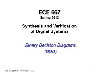
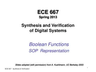
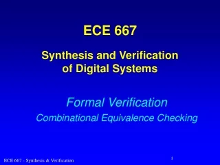
ECE 667 Spring 2011 Synthesis and Verification of Digital Systems

1. ECE 667Spring 2011Synthesis and Verificationof Digital Systems FSM Traversal ECE 667 - Synthesis & Verification

2. O X (s,x) (s,x) s s’ R Finite State Machine (FSM) Model • FSM M(X,S, , ,O) • Inputs: X • Outputs: O • States: S • Next state function, (s,x) : S  X  S • Output function, (s,x) : S X  O ECE 667 - Synthesis & Verification

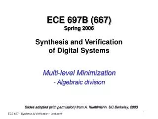
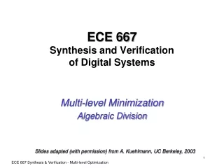
3. 1/0 0/1 s0 s1 s2 1/0 0/1 FSM Traversal • State Transition Graphs • directed graphs with labeled nodes and arcs (transitions) • symbolic state traversal methods • important for symbolic verification, state reachability analysis, FSM traversal, etc. 0/0 ECE 667 - Synthesis & Verification

4. Existential Quantification • Existential quantification (abstraction) xf = f |x=0+ f |x=1 • Example: x(x y + z) = y + z • Note: xf does not depend on x (smoothing) • Useful in symbolic image computation (deriving sets of states) ECE 667 - Synthesis & Verification

5. Existential Quantification - cont’d • Function can be existentially quantified w.r.to a vector: X = x1x2… Xf = x1x2...f = x1 x2 ...f • Can be done efficiently directly on a BDD • Very useful in computing sets of states • Image computation: next states • Pre-Image computation: previous states from a given set of initial states ECE 667 - Synthesis & Verification

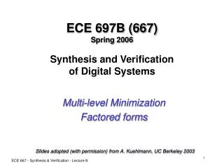
6. R(u,v) S(u) Img(v) Image Computation • Computing set of next states from a given initial state (or set of states) Img( S,R ) = uS(u)• R(u,v) • FSM: when transitions are labeled with input predicates x, quantify w.r.to all inputs (primary inputs and state var) • Img( S,R ) = x uS(u)• R(x,u,v) ECE 667 - Synthesis & Verification

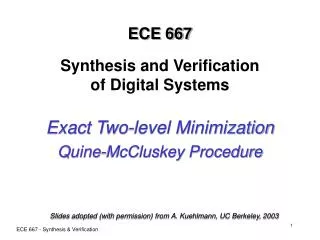
7. s2 a a xy XY 01 s1 s4 1 00 01 0 00 10 - 10 11 ………. 00 a’ 11 10 s3 Image Computation - example Compute a set of next states from state s1 • Encode the states: s1=00, s2=01, s3=10, s4=11 • Write transition relations for the encoded states: R = (ax’y’X’Y + a’x’y’XY’ + xy’XY + ….) ECE 667 - Synthesis & Verification

8. s2 a 01 s1 s4 00 a’ 11 10 s3 Example - cont’d • Compute Image from s1 under R Img( s1,R ) = a xy s1(x,y) • R(a,x,y,X,Y) =a xy(x’y’)• (ax’y’X’Y + a’x’y’XY’ + xy’XY + ….) = axy(ax’y’X’Y + a’x’y’XY’ ) = (X’Y + XY’ ) = {01, 10} = {s2, s3} Result: a set of next states for all inputs s1  {s2, s3} ECE 667 - Synthesis & Verification

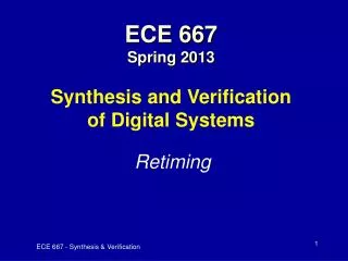
9. Pre-Image Computation • Computing a set of present states from a given next state (or set of states) Pre-Img( S’,R) = vR(u,v) )• S’(v) R(u,v) S’(v) Pre-Img(u) • Similar to Image computation, except that quantification is done w.r.to next state variables • The result: a set of states backward reachable from state set S’, expressed in present state variables u • Useful in computing CTL formulas: AF, EF ECE 667 - Synthesis & Verification