Download
1 / 40
400 likes | 569 Views
Design of an Agent-Based Computational Economics Approach to Forecasting Future Freight Flows for the Chicago Region. Prepared for: TRB SHRP 2 C43 Symposium on Innovations in Freight Modeling & Data . Prepared by: John Gliebe, RSG, Inc. (Presenter) Kermit Wies , CMAP

E N D
Design of an Agent-Based Computational Economics Approach to Forecasting Future Freight Flows for the Chicago Region Prepared for: TRB SHRP 2 C43 Symposium on Innovations in Freight Modeling & Data Prepared by: John Gliebe, RSG, Inc. (Presenter) Kermit Wies, CMAP Colin Smith, RSG, Inc. Kaveh Shabani, RSG, Inc. Maren Outwater, RSG, Inc.
Overview • Background and motivation • Agent-based computational economics • Overview of current model system • Overview of proposed model design • Procurement market game • Next steps
Background • The Chicago Metropolitan Agency for Planning (CMAP) has recently developed a two-tiered modeling system to analyze regional freight traffic • Original work: FHWA BAA Research project (2011), Cambridge Systematics, University of Illinois-Chicago, RSG, Inc. • Address complexities of freight modeling: commodities produced and consumed, local pick-up and delivery, warehousing and tour formation • The first tier is referred to as the “mesoscale model” or “national supply chain model” and represents freight flows between the CMAP region and the rest of the U.S. • The second tier model operates within the region, modeling local freight-hauling truck movements using a tour-based microsimulation and has been dubbed the “microscale model” or the “tour-based truck model” • Commodity flows, including future freight flows, are derived from those found in the Freight Analysis Framework, Version 3 (FAF3) data products, developed by the Federal Highway Administration (FHWA).
Motivation • For policy and planning sensitivity analysis, CMAP would like a tool to systematically vary forecasts to reflect: • Potential changes in macroeconomic conditions (e.g., foreign trade levels, price of crude oil); • Large-scale infrastructure changes (e.g., port expansions, new intermodal terminals); • Technological shifts in logistics and supply chain practices (e.g., near-sourcing, out-sourcing, productivity enhancements); and • Other assumptions and scenario inputs related to the economic competitiveness of the Chicago region and its infrastructure investments. To support these objectives… • Future freight forecasts will need to be produced endogenously—focus on producer sourcing decisions to meet production levels • Foreign trade and macroeconomic conditions will need to included in the producer sourcing decisions • Price signals—transport and logistics costs and other costs will need to be part of sourcing decisions
Theoretical Drivers Behind Approach • Supply chain decisions are made by individuals on behalf of the companies for whom they work, characterized by: • Imperfect information • Cultural baggage • Personal affinity for particular business partners • Limited search efforts based on custom, imitation, satisficing behavior • Purchasing agents want to save costs and selling agents want to maximize revenues, but It may not be realistic to assume that agents will make mathematically optimal decisions • Variation in value systems across markets (examples): • Emphasize cost savings for bulk commodities with low storage costs • Emphasize frequency of shipments for perishable commodities • Practice vertical integration (in-house sourcing) for complex commodities, such as components of high-precision medical equipment • Variation in market mechanisms • Ad hoc bi-lateral agreements • Auctions and bidding • Collusions, side agreements • Varying levels of competition
What is agent-based computational economics? • ACE research characterized by rigorous study of economic systems through computational experiments • “Bottom up” approach in which individual agents are simulated in a virtual world in which they make decisions, interactwith and react to each other, and patterns emergefrom the collective actions of many agents • Interactions between agents typically take the form of cooperation games • Methodological kinship with complex systems studies in social and natural sciences • Electric power trading • Social choice and voting • Racial segregation in housing • School choice • Habitat destruction • Honeybee swarms Source of graphic: http://computationallegalstudies.com/2010/07/27/agents-of-change-agent-based-models-and-methods-the-economist/
ACE: Answering questions about complex systems • Why have certain global regularities emerged and persisted despite the absence of centralized planning and control, while other global outcomes have not been observed? • How are trends in supply-chain and logistics practices, such as insourcing, outsourcing, and near-sourcing influenced by privately held values and beliefs regarding various forms of uncertainty, asset specificity, and commodity attributes? • How much is simply imitation? • What types of micro-level dynamics of individual traders lead to the collective patterns market behavior that we observe? • Which agents in the supply chain network have the greatest influence on other agents (commodities, industries)? • Are there ties between agent/industries that may be important to assessing regional competitiveness and the likely trends in future freight flows? • How can good economic (infrastructure) policies be designed to achieve their intended effect? • Road pricing, traffic flow management, trade tariffs, port capacity expansions
Current Mesoscale Freight Model • Synthesizes a list of businesses in Chicago, the rest of the US, and an international sample • Connects suppliers to buyers based on the commodities produced by the supplier and consumed by the buyer • Distributes commodity flows amongst the paired suppliers and buyers National Scale • For each buyer/supplier pair, selects whether shipments are direct or involve intermediate handling (intermodal, distribution center) • For each buyer/supplier pair, converts an annual commodity flow to shipments by size and frequency • Identifies the mode for each leg of the trip from supplier to buyer and the transfer locations Regional Scale • The local deliveries and picks up in the Chicago area are simulated using a truck touring model
Major Changes to Mesoscale Model Design • Adding attributes to describe firms/establishments, based on operating typologies • Commodity flow data no longer basis for predictions, but used in calibration and testing as benchmarks • Business linkages, shipment demand, and mode determined through a joint decision framework, based on the outcome of agent-based simulations • Outcome are shipments that feed directly into the truck touring model (simulation of delivery and pickup)
Synthesize Firms • Start with existing method of firm synthesis • Within the CMAP region, firms are treated as establishments in that they are situated in a single location and function as establishments • Outside of the CMAP region, “representative” firms will be created to represent a single industry, and region/country (FAF zone) • E.g., Wyoming Coal Producers • Firm attributes • Industry Code (NAICS) • CPB Zone (County Business Patterns zone used during supplier selection) • FAF Zone (country/region) • CMAP modeling zone • Commodity Type(s) Produced (SCTG) • Size (number of employees) • Production capacity (commodity units produced per year)
Assign Firm Types and Preferences • Purpose to define firms’ sourcing preferences (tradeoffs) for various combinations of source offerings (“attribute bundles”) • Commodity Service Offerings • Unit cost / total cost • Average shipment time • Frequency of shipments / Average shipment size • Proximity of supplier • Perceived reliability of the supplier • Perceived quality of the supplier’s commodity (assert for certain scenarios) • Firm Operational Types • Efficiency vs. Responsiveness: Is commodity “innovative” or “functional”? • Geographic Proximity: Are there preferences for near-sourcing vs. far-sourcing? • Centralization Tendencies: Is commodity likely to utilize warehousing and distribution systems? • Vertical Integration Tendencies: Is commodity likely to be produced in-house?
Assign Firm Commodity Production Levels • U. S. Bureau of Economic Analysis (BEA) data will be used to estimate the total dollar-value of output commodities based on firm size • Account for production cost differences for non-U.S. countries • For imports, BEA reports producer prices at U.S. port of entry in U.S. dollars
Calculate Input Procurement Requirements • BEA Input-Output (I-O) tables • “Use” tables after redefinitions to represent only direct inputs • Normalized becomes Direct Requirements table (partial table shown)
Estimate Transport and Non-Transport Costs • Transport and Logistics Costs • Use skims from the multi-modal network model and unit costs created as part of the current mesoscale model to provide transport and logistics costs, composed of: • Ordering cost • Transport and handling cost • Damage cost • Inventory in-transit cost • Carrying cost • Safety stock cost • Total Costs • Use FAF3estimates of total shipment values between FAF zones to provide a total cost figure • Non-Transport/Logistics Costs = Total Costs – Transport Costs
Match Buyers and Sellers, Bundling Service Attributes • Create buyer agents with preferences for bundled cost-service attributes • For each of the 43 commodity types under consideration, a procurement market model will be run • This is done through a “procurement market game” • The objective of this step is to find suppliers for every commodity input required by buyers • Outcome is joint choice of supplier, shipment size, distribution center use and mode-path
Procurement Market Game (PMG) • Research literature in supply chain sourcing decisions focuses on auction mechanisms that can be used to optimize outcomes • E-procurement systems require efficient, robust algorithms (algorithmic game theory) • Common objectives are to induce suppliers to bid at true cost, avoid collusion, and other forms of strategic lying • Example: “2nd Price Sealed Bid” (Vickery 1961) • Appropriateness of auction mechanisms for Mesoscale Freight Model • Industry and commodity-specific • Not necessarily applicable to smaller and less technologically advanced firms • Typically designed for optimization • Won’t necessarily capture idiosyncratic behavior of agent preferences, habits and beliefs • ACE approaches offer a more general, flexible framework • PMG inspired by Trade Network Game (TNG) (Tesfatsion, McFadzean, Iowa State U.) • Agents are buyers, sellers and dealers (buy or sell) • 2 x 2 Payoff matrix – “cooperate” or “defect” labeling (e.g., Prisoners Dilemma) • Evolutionary programming framework (genetic algorithm) • Multiple rounds of pairwise trades • Agent expectations about other trading partners are updated after each round based on outcomes of all pairwise trading games • Market properties emerge through iterative play
Initializing Agents • Buyer Attributes • NAICS • Size (# employees) • FAF Zone • Output commodity • Input commodity • Input commodity requirements ($ annual purchase) demand • Seller Attributes • NAICS • Size (# employees) • FAF Zone • Output commodity • Production level ($ annual output) capacity B S • Seller Cost-Service Bundle • Shipment sizes • Average shipping times • Distribution centers • Mode • Cost • Buyer Preferences • Efficient vs. Responsive • Near-source vs. Far-source • Centralized Distribution • Vertical Integration
Round 1 B B B B B S S S
Round 2 B B B B B S S S
Round 3 B B B B B S S S
Example PMG: Trade Scenario “A” • Large buyer “L” and a small buyer “S” who are both in the packaged foods industry, commodity code, CC=1 • Each buyer needs to purchase a quantity of an input commodity, seafood, commodity code, CC=2. Both buyers are in the geographic zone, GZ=1 • Three sellers: foreign (‘F”), domestic (“D”), and local (“L”), each offering different bundles of unit costs and shipping time
Pairwise Trade L-F • Large Buyer and Foreign Seller
Pairwise Trade S-D • Small Buyer and Domestic Seller
Pairwise Trade L-L • Large Buyer and Local Seller
Scenario A Resolution • And so on… All pairwise combinations (2 x 3 = 6) are calculated and expected payoffs for each game are updated based on these pairwise outcomes • Only partnership formed was between Buyer L ("large") and Seller L ("local"). • Under an assumption of mutual exclusivity, an initially favorable L-D match was superseded by L-L (slightly better for the buyer) • Buyer S ("small") was outbid after holding out for the preferred provider ("local"). • Buyer S was rejected by all of the sellers, who were holding out for Seller L ("large"). • During the second round, buyers and sellers would update their beliefs about the probability of a successful trade, which should result in a second alliance forming between Buyer S and Seller D ("domestic"). • Seller F ("foreign") is priced out of this market for fish, but could become competitive in a different scenario if cost structures or preferences were to change.
Expectations of PMG • Replicating what actually goes on in a procurement market is challenging • Different payoff matrices may be defined to capture different styles and assumptions on the bilateral trade, resulting in different emergent behavior • We may create 3-5 general types of games to represent commodity markets of similar types • Buyers will outnumber sellers in the majority of markets • Pair-feasibility criteria will be developed • Stopping criteria to be determined, but providing suppliers to fulfill every buyer’s input needs will be minimum—convergent solutions preferred • Sellers will have capacity constraints • Some buyers will want to spread risk and choose multiple sellers • Cost structure assumptions and parameters, and utility preference weights will be highly influential, thus a large part of the development time • FAF3 flows will be used for benchmarking and calibration of aggregate results
Planned Scenario Testing • Impacts of full implementation of Chicago's CREATE program • Impacts of implementation of Midwest Intermodal Hub in Iowa • Impacts of expansion of Port of Prince Rupert, BC • Impacts of reduction/increase in U.S. Trade with China Source: http://www.createprogram.org/linked_files/ProjectMap_print.pdf
Next Steps • Development of PMG test bed (ongoing) • Incremental testing of variables, algorithms and assumptions • Assess convergence properties, reasonableness of results, computational time, realism of portrayed competition • Start with single commodity procurement market; gradually try additional markets, look for commonalities and generalizability • Start with simpler single-cost variables in payoffs, gradually add other variables • Test different utility weighting parameter values • Test full combinatorial treatment vs. filtering and sampling • Experiment with assumptions information known to agents • Experiment with other algorithmic assumptions
San Diego Evansville Kermit Wies CMAP kwies@cmap.illinois.gov 312-386-8820 John Gliebe RSG john.gliebe@rsginc.com 240-283-0633 Kaveh Shabani RSG kaveh.shabani@rsginc.com 801-736-4100 Colin Smith RSG colin.smith@rsginc.com 802-295-4999 Maren Outwater RSG maren.outwater@rsginc.com 414-446-5402 Craig Heither CMAP cheither@cmap.illinois.gov (312) 386-8768 www.rsginc.com 31
Firm Synthesis Firms are synthesized for the entire U.S. with a high level of industrial sector detail, and across several employment size categories Data: County Business Patterns: business establishments by employment size category and industrial sector for each county Input/output data(US BEA) to tag each establishment with the commodity that it produces/consumes (interested in the commodities that require transportation)
Application Development in R • Hardware • Manufacturer: HP Z200 Workstation • Processor: Intel Core i7 CPU 870 @ 2.93 GHz • Installed RAM: 12.0 GB • OS: Windows 7 Professional (64-bit) • Scripting Software • R version 2.14 • Runtime • Total run time is 80-90 minutes
Cost Function (Current Mesoscale mode, improved equation) Ordering Cost Transport and Handling Cost Inventory in-transit cost Damage Cost Carrying Cost Safety Stock Cost (source: Cambridge Systematics, 2011)
Levels of Response Sensitivity in Forecasting • Different levels of response sensitivity can be incorporated in the model design (not mutually exclusive) Stimulus: Change in price of an input commodity “A” 1. Switch suppliers for input commodity “A”? Part of model’s basic response set-PMG Requires budget-awareness. Would need to be sub-problem within PMG. Perhaps too complex –defer to future 2. Switch suppliers for input commodity “B”? 3. Pass cost change along in price of output commodity? Supply chain activity network propagation 4. Cost is “global” and changes factors of production? Change I-O coefficients? Change output levels? Change in final demand?
“Stone mining/quarrying” (1st, 2nd order ties) Stone mining & quarrying
“Stone mining/quarrying” (1st, 2nd, 3rd order ties) Iron and steel ferrous alloys Stone mining & quarrying