Download
1 / 22
220 likes | 250 Views
Explore MINERVA's advanced features like 3D E&M fields, particle dynamics, and simulation algorithms for X-Ray FELs. Understand MINERVA's inputs, outputs, and parallelization for efficient design evaluation.

E N D
Paper presented at the Workshop on Designing Future X-Ray FELs Daresbury Laboratory, England 31 August – 2 September 2016 THE MINERVA FEL SIMULATION CODE H.P. Freund,1P.J.M. van der Slot,1,2 D. Grimminck,3 I. Setija,3 P. Falgari,4 D. Dunning,5 and N. Thompson5 1Colorado State University, Fort Collins, CO, USA 2Mesa+ Institute for Nanotechnology, University of Twente, Enschede, the Netherlands 3ASML B.V., Veldhoven, the Netherlands 4LIME B.V. Eindhoven, the Netherlands 5STFC Daresbury Laboratory, Warrington, UK
MINERVA OVERVIEW – E&M FIELDS • 3D E&M FIELDS • Polychromatic SVEA approximation • Time-dependent and/or polychromatic physics • Gaussian Modal decomposition of the fields extremely low memory requirement • Planar, Helical, or Elliptic polarizations • Adaptive eigenmode expansion (SDE) for field propagation minimizes the number of modes • Slippage can be applied at arbitrary intervals
MINERVA OVERVIEW- PARTICLES • Particle dynamics are treated from first principles (not KMR) • Internal field models for Planar (FPF & PPF), Helical, and APPLE-II Undulators • The JJ-factor is implicitly included for planar & elliptic undulators • The undulator field can be imported from a 3D field map • Internal models for quadrupoles and dipoles (chicanes) • Harmonics & sidebands implicitly included • Start-up from noise (Fawley algorithm)/Prebunched beam
MINERVA OVERVIEW- ALGORITHM • Numerical Approach • Runge-Kutta Integration of particle and field equations simultaneously • 6Nparticles + Nharmonics(2Nmodes + 2) ODE (equations) per slice • Must use 20 – 30 steps/undulator period to resolve wiggle-motion • Can use either 2nd or 4th order Runge-Kutta • Fortran 90/95 with MPI – dynamic memory allocation • Portable – LINUX, WINDOWS, MAC OS • Flexible - Can easily add new features for Engineering Design Evaluation • New wiggler/beam models – Variable polarization states
MINERVA INPUTS • INPUTS • Magnetostatic Fields – undulators, quadrupoles, dipoles • Specify start/end positions & field strengths • Adiabatic transitions between the fields and free-space • Free-space drift is assumed in the gaps between the fields • Electron Beam • Internal Gaussian beam with top-hat, parabolic, or Gaussian temporal profile • Import a beam file derived from beam dynamics codes • Provide the detailed Twiss parameters for each slice • Shot-noise or prebunched beam phases added • Translators for ELEGANT, DIMAD, and PARMELA • Import a GENESIS-type distribution file • Import actual particles directly – work in progress • Optical Field • Specify harmonic number, mode numbers, power, type (Hermite/Laguerre), etc.
MINERVA OUTPUTS • OUTPUTS – text files (no graphical output) • Principal outputs – Optical Energy and/or Power vs z files • Beam evolution vs z (per slice or average)/phase space dumps at designated points • Spectra (FFTs) and optical temporal profiles at designated points • Transverse fluence at designated points (for each slice or average) • Spent beam distributions • Transverse field on a grid for propagation using OPC
MPI PARALLELIZATION • MINERVA is parallelized using the Message Passing Interface and Fortran 90/95 • Transportable: Macintosh, Windows, Linux Sample MINERVA Run • Run times may vary, but the scaling with the number of CPU’s on a cluster is efficient
APPLE-II UNDULATOR MODEL We model an APPLE-II undulator using a super-position of two crossed planar undulators with a relative phase shift f Valid near the axis of symmetry The ellipticity is given by: 0 £f < p/2 p/2 £f£p
MINERVA SIMULATION • MINERVA simulations for SPARC-like parameters show a decrease in the gain length and increase in the saturation distance with decreasing ellipticity – as expected. • MINERVA is in reasonable agreement with the Ming Xie formulae that have been generalized to include the new resonant wavelength and JJ-factor. J.R. Henderson, L.T. Campbell, H.P. Freund, B.W.J. McNeil, New J. Phys. 18, 062003 (2016)
LCLS SIMULATION – GAIN TAPER • The actual magnet strengths and positions are used in MINERVA including the undulators and FODO lattice for both the gain & saturation tapers. Gain Taper Saturation Taper Beam transport is quite uniform • The undulator field strengths are taken from the actual values for the gain & saturation tapers.
LCLS – GAIN & SATURATION TAPER • MINERVA simulations (25 noise seeds) of the original LCLS with the gain taper have shown good agreement with the data. • The gain taper is still a taper and we see a small positive slope. • Question: Neither ICR nor wakefields have been included – are they necessary? 8% discrepancy Data courtesy: H.-D. Nuhn • MINERVA is in reasonable agreement with the saturation taper data for a range of beam parameters. Data courtesy: D. Ratner
SPARC SIMULATION MINERVA is in good agreement with the SPARC experimental data. Reference: L. Giannessi et al., Phys. Rev. ST-AB 14, 060712 (2011)
BNL TAPERED AMPLIFIER • MINERVA was validated for an IR, tapered amplifier exp’t. at Brookhaven National Laboratory – good agreement found tapered uniform experiment MINERVA • Reasonable agreement also found for the output spectrum and 3rd harmonic power. Ref.: X.J. Wang, H.P. Freund, W. Miner, J. Murphy, H. Qian, Y. Shen, and X. Yang,, Phys. Rev. Lett. 103, 154801 (2009)
OSCILLATOR SIMULATION electron beam wiggler • Interfaces written between MINERVA/OPC • MINERVA simulates the interaction in the wiggler and writes the complex phase front at the wiggler exit to a file that is handed off to OPC • OPC propagates the field around the resonator and hands off the complex phase front at the wiggler entrance to MINERVA OPC Upstream OPC Downstream • MINERVA writes the phase front at the output of the wiggler directly into the input file for OPC, but uses a translator to decompose the complex phase front at the wiggler entrance from OPC back into Gaussian optical modes and then write a new input file. This procedure has been used to simulate low-gain oscillators and regenerative amplifiers with hole out-coupling MINERVA Input MINERVA Output
THE JLAB 10kW UPGRADE Electron Beam Beam Energy: 115 MeV Bunch Charge: 115 pC Bunch Length: 390 fsec Bunch Frequency: 74.85 MHz Emittance: 9 mm-mrad (wiggle plane), 7 mm-mrad Energy Spread: 0.3% Wiggler Period: 5.5 cm Amplitude: 3.75 kG Length: 30 periods Radiation/Resonator Wavelength: 1.6 microns Resonator Length: 32 m Rayleigh Range: 0.75 m Out-Coupling: 21% (transmissive) • The experiment recorded an average output power of 14.3 ± 0.72 kW. • Earlier simulation with MEDUSA/OPC was in good agreement and found an average output power of 12.3 kW [reference: P.J.M. van der Slot et al., Phys. Rev. Lett. 102, 244802 (2009)]. • MINERVA/OPC is also in good agreement and finds an average output power of 14.4 kW.
SHOT-NOISE SIMULATION • Despite the fact that many codes (GINGER, GENESIS, MEDUSA, MINERVA) employ the Fawley algorithm [Phys. Rev. ST-AB 5, 070701 (2002)] for setting up the initial shot noise distribution, there are substantial differences between the codes regarding the magnitude of the start-up noise. Giannessi et al., Phys. Rev. ST-AB 14, 00712 (2011) Huang & Kim, Phys. Rev. ST-AB 10, 034901 (2007) • We no longer believe that this explanation holds across all the codes
GENESIS – MINERVA COMPARISON • We have compared MINERVA & GENESIS directly for a given undulator configuration using an initial particle distribution created by GENESIS • In this case the start-up noise predicted by the two codes is very similar, despite the differences in the E&M solvers between the codes OPEN QUESTION: What is the source of the discrepancy when the internal particle loads are used in each code?
SUMMARY • MINERVA includes multiple configurations: • Amplifiers • SASE • Oscillators/Regenerative Amplifiers (with OPC) • Optical Klystrons & HGHG by including chicanes in the transport line • MINERVA averages the wave equation (SVEA) but not the orbit equations • Input actual fields and positions – entry/exit tapers • MINERVA capabilities: • Multiple optical polarizations • Planar, Helical, Elliptic • Harmonics included self-consistently • Multiple undulator configurations • Planar, Helical, APPLE-II (variable polarization), Field Map • Segmented undulators with FODO lattice and/or chicanes • MINERVA has been extensively validated by comparison with experiments • MINERVA is written in Fortran 90/95 • Dynamic memory management (relatively small memory footprint) • Parallelization with MPI is efficient • Transportable - platform independent (Linux, Mac OS, Windows)
MINERVA FORMULATION: z z + Dz For each slice, MINERVA integrates a system of ODE’s for N particles and M modes in going from z z + Dz. All of the terms on the RHS must be calculated for each step before the Runge-Kutta algorithm (2nd or 4th Order) can push each of the variables. Sums over Modes for each Particle There are always more particles than modes Sums over Particles for each Mode
SLIPPAGE APPLICATION • MINERVA applies slippage by interpolating the amount of slippage between adjacent optical slices over any desired interval in z. • The default option is to apply slippage every step in z (20 – 30 times/lw). This is a nearly continuous process that allows the electron phase space to evolve adiabatically. • It is also possible to apply slippage in a stepwise manner .If there are N wavelengths between slices, then slippage is often applied every 10 undulator periods. For SASE, this can result in a sudden change in the phase space behavior of the electron beam if an optical slice with a markedly different power advances into a succeeding electron slice. If the phase space area enclosed by the separatrix changes suddenly, then electrons may switch between trapped and untrapped orbits. This is an unphysical situation that imparts a kick to the phase space.
THE JJ-FACTOR • The elliptic undulator alters the effective K-value and, hence the resonance condition • The JJ-factor becomes The variation in the undulator field and JJ-factor for a fixed resonant wavelength is shown to the right J.R. Henderson, L.T. Campbell, H.P. Freund, B.W.J. McNeil, New J. Phys. 18, 062003 (2016)