Download
1 / 37
370 likes | 553 Views
Review of the IOOS Super-Regional Modeling Testbed Progress: Estuarine Hypoxia Modeling OUTLINE. Intro: Participants, motivation Methods: ( i ) Models, (ii) observations, (iii) skill metrics Results ( i ): What is the relative hydrodynamic skill of these CB models?

E N D
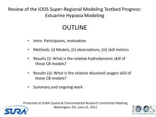
Review of the IOOS Super-Regional Modeling Testbed Progress: Estuarine Hypoxia Modeling OUTLINE • Intro: Participants, motivation • Methods: (i) Models, (ii) observations, (iii) skill metrics • Results (i): What is the relative hydrodynamic skill of these CB models? • Results (ii): What is the relative dissolved oxygen skill of these CB models? • Summary and ongoing work Presented atSURA Coastal & Environmental Research Committee Meeting Washington, DC, June 21, 2011
Review of the IOOS Super-Regional Modeling Testbed Progress: Estuarine Hypoxia Modeling Carl Friedrichs(VIMS) and the Estuarine Hypoxia Testbed Team • Federal partners (*unfunded partner) • David Green* (NOAA-NWS) – Transition to operations at NWS • Lyon Lanerole (NOAA-CSDL) – Transition to operations at CSDL; CBOFS2 • Lewis Linker* (EPA), Carl Cerco* (USACE) – Transition to operations at EPA; CH3D, CE-ICM • Doug Wilson* (NOAA-NCBO) – Integration w/observing systems at NCBO/IOOS • Non-federal partners • Marjorie Friedrichs, Aaron Bever(VIMS) – Metric development and model skill assessment • Ming Li, Yun Li (UMCES) – UMCES-ROMS hydrodynamic model • Wen Long, Raleigh Hood (UMCES) – ChesROMS with NPZD water quality model • Scott Peckham (UC-Boulder) – Running multiple ROMS models on a single HPC cluster • Malcolm Scully (ODU) – ChesROMS with 1 term oxygen respiration model • Kevin Sellner (CRC) – Academic-agency liason; facilitator for model comparison • JianShen (VIMS) – SELFE, FVCOM, EFDC models • John Wilkin, Julia Levin (Rutgers) – ROMS-Espresso + 7 other MAB hydrodynamic models Presented atSURA Coastal & Environmental Research Committee Meeting Washington, DC, June 21, 2011
Motivation for Studying Estuarine Hypoxia (VIMS, ScienceDaily) (UMCES, Coastal Trends)
Motivation (cont.): Existing paradigm is that salinity stratification must be modeled well to predict hypoxia well. Mid-summer oxygen differences across the pycnocline versus salinity difference for mid-Cheseapeake Bay stations, 1949-1980 (Flemer et al. 1983; Boicourt et al. 1992).
Review of the IOOS Super-Regional Modeling Testbed Progress: Estuarine Hypoxia Modeling in Chesapeake Bay OUTLINE • Intro: Participants, motivation • Methods: (i) Models, (ii) observations, (iii) skill metrics • Results (i): What is the relative hydrodynamic skill of these CB models? • Results (ii): What is the relative dissolved oxygen skill of these CB models? • Summary and ongoing work Presented atSURA Coastal & Environmental Research Committee Meeting Washington, DC, June 21, 2011
Methods (i) Models (cont.): 5 Dissolved Oxygen Models (so far) • ICM: CBP model; complex biology • bgc: NPZD-type biogeochemical model • 1eqn: Simple one equation respiration (includes SOD) • 1term-DD: depth-dependent net respiration • (not a function of x, y, temperature, nutrients…) • 1term: Constant net respiration
Methods (i) Models (cont.): 5 Dissolved Oxygen Models (so far) • ICM: CBP model; complex biology • bgc: NPZD-type biogeochemical model • 1eqn: Simple one equation respiration (includes SOD) • 1term-DD: depth-dependent net respiration • (not a function of x, y, temperature, nutrients…) • 1term: Constant net respiration • CH3D + ICM • EFDC + 1eqn, 1term • CBOFS2 + 1term, 1term+DD • ChesROMS + 1term, 1term+DD, bgc Methods (i) Models (cont.): 8 Multiple combinations (so far)
Methods (ii) observations: S and DO from Up to 40 CBP station locations Data set for model skill assessment: ~ 40 EPA Chesapeake Bay stations Each sampled ~ 20 times in 2004 Temperature, Salinity, Dissolved Oxygen Map of Late July 2004 Observed Dissolved Oxygen [mg/L] (http://earthobservatory.nasa.gov/Features/ChesapeakeBay)
How do we compare these models to data and to each other? • e.g., Is ChesROMS 1-Term (very simple) or CH3D-ICM (very complex) more accurate? • e.g., Which is modeled better, dissolved oxygen (DO) or salinity stratification (dS/dz)? (from A. Bever)
Methods (iii) Skill Metrics: Target diagram (modified from M. Friedrichs)
Review of the IOOS Super-Regional Modeling Testbed Progress: Estuarine Hypoxia Modeling in Chesapeake Bay OUTLINE • Intro: Participants, motivation • Methods: (i) Models, (ii) observations, (iii) skill metrics • Results (i): What is the relative hydrodynamic skill of these CB models? • Results (ii): What is the relative dissolved oxygen skill of these CB models? • Summary and ongoing work Presented atSURA Coastal & Environmental Research Committee Meeting Washington, DC, June 21, 2011
Results (i): Hydrodynamic Model Comparison bias [psu] (a) Bottom Temperature bias [°C] (b) Bottom Salinity Inner circle in (a) & (b) = error from CH3D model • All models do very well hind-casting temperature. • All do well hind-casting bottom salinity with CH3D and EFDC doing best. unbiased RMSD [psu] unbiased RMSD [°C] • Stratification is a challenge for all the models. • All underestimate strength and variability of stratification with CH3D and EFDC doing slightly better. • CH3D and ChesROMS do slightly better than others for pycnocline depth, with CH3D too deep, and the others too shallow. • All underestimate variability of pycnocline depth. bias [psu/m] bias [m] (c) Stratification at pycnocline Outer circle in each case = error from simply using mean of all data (d) Depth of pycnocline unbiased RMSD [psu/m] unbiased RMSD [m] (from A. Bever, M. Friedrichs)
Results (i) Hydrodynamics: Temporal variability of stratification at 40 stations CH3D ChesROMS • Model behavior for stratification is similar in terms of temporal variation of error at individual stations EFDC CBOFS2 Mean salinity of individual stations [psu] UMCES-ROMS (from A. Bever, M. Friedrichs)
Results (i) Hydrodynamics: Temporal variability of depth of pycnocline at 40 stations CH3D ChesROMS • Model behavior for pycnocline depth is also similar in terms of temporal variation of error at individual stations EFDC CBOFS2 Mean salinity of individual stations [psu] UMCES-ROMS (from A. Bever, M. Friedrichs)
Results (i) Hydrodynamics (cont.): Sensitivity to model refinement • Used 4 models to test sensitivity of hydrodynamic skill to: • Vertical grid resolution (CBOFS2) • Freshwater inflow (CBOFS2; EFDC) • Vertical advection scheme (CBOFS2) • Atmospheric forcing – winds (ChesROMS; EFDC) • Horizontal grid resolution (UMCES-ROMS) • Coastal boundary condition (UMCES-ROMS) • 2004 vs. 2005 (in progress)
Results (i) Hydrodynamics (cont.): Sensitivity of pycnocline depth CBOFS2 0.2 -0.6 -0.2 -0.4 -0.8 -0.2 -0.2 (from A. Bever, M. Friedrichs) CBOFS2model pycnocline depth is insensitive to: vertical grid resolution, vertical advection scheme and freshwater river input
Results (i) Hydrodynamics (cont.): Sensitivity of stratification at pycnocline Stratification (from A. Bever, M. Friedrichs) CH3D, EFDC ROMS Stratification at pycnocline is not sensitive to horizontal grid resolution or changes in atmospheric forcing. (Stratification is still always underestimated)
Results (i) Hydrodynamics (cont.): Sensitivity of bottom salinity Bottom Salinity High horiz res Low horiz res Bottom salinity IS sensitive to horizontal grid resolution (from A. Bever, M. Friedrichs)
Review of the IOOS Super-Regional Modeling Testbed Progress: Estuarine Hypoxia Modeling in Chesapeake Bay OUTLINE • Intro: Participants, motivation • Methods: (i) Models, (ii) observations, (iii) skill metrics • Results (i): What is the relative hydrodynamic skill of these CB models? • Results (ii): What is the relative dissolved oxygen skill of these CB models? • Summary and ongoing work Presented atSURA Coastal & Environmental Research Committee Meeting Washington, DC, June 21, 2011
Results (ii): Dissolved Oxygen Model Comparison • Simple models reproduce dissolved oxygen (DO) and hypoxic volume about as well as more complex models. • All models reproduce DO better than they reproduce stratification. • A five-model average does better than any one model alone. (from A. Bever, M. Friedrichs)
Results (ii): Dissolved Oxygen Model Comparison (cont.) (from A. Bever, M. Friedrichs)
Results (ii): Dissolved Oxygen Model Comparison (cont.) Average of these 5 models is better than any single model. Hypoxic Volume in km3
Results (ii) Dissolved Oxygen: Temporal variability of bottom DO at 40 stations 1-term DO model ICM (most complex model) ChesROMS-1term (simplest model) Mean bottom DO individual stations [mg/L] Total RMSD = 0.9 ± 0.1 Total RMSD = 0.9 ± 0.1 1-term DO model underestimates high DO and overestimates low DO: high not high enough, low not low enough (from A. Bever, M. Friedrichs)
Results (ii) Dissolved Oxygen: Top-to-Bottom DS and Bottom DO in Central Chesapeake Bay • ChesROMS-1term • model • All models reproduce DO better than they reproduce stratification. • So if stratification is not controlling DO, what is? (by M. Scully)
Results (ii) (cont.): Effect of Physical Forcing on Dissolved Oxygen ChesROMS-1term model 20 10 0 Base Case Hypoxic Volume in km3 Jan Feb Mar Apr May Jun Jul Aug Sep Oct Nov Dec Date in 2004 (by M. Scully) (by M. Scully)
Results (ii) (cont.): Effect of Physical Forcing on Dissolved Oxygen ChesROMS-1term model 20 10 0 Base Case Hypoxic Volume in km3 Freshwater river input constant Jan Feb Mar Apr May Jun Jul Aug Sep Oct Nov Dec Date in 2004 Seasonal changes in hypoxia are not a function of seasonal changes in freshwater. (by M. Scully) (by M. Scully)
Results (ii) (cont.): Effect of Physical Forcing on Dissolved Oxygen ChesROMS-1term model 20 10 0 July wind year-round Base Case Hypoxic Volume in km3 Jan Feb Mar Apr May Jun Jul Aug Sep Oct Nov Dec Date in 2004 Seasonal changes in hypoxia may be largely due to seasonal changes in wind. (by M. Scully) (by M. Scully)
Results (ii) (cont.): Effect of Physical Forcing on Dissolved Oxygen ChesROMS-1term model 20 10 0 Base Case Hypoxic Volume in km3 January wind year-round Jan Feb Mar Apr May Jun Jul Aug Sep Oct Nov Dec Date in 2004 Seasonal changes in hypoxia may be largely due to seasonal changes in wind. (by M. Scully) (by M. Scully)
Review of the IOOS Super-Regional Modeling Testbed Progress: Estuarine Hypoxia Modeling OUTLINE • Intro: Participants, motivation • Methods: (i) Models, (ii) observations, (iii) skill metrics • Results (i): What is the relative hydrodynamic skill of these CB models? • Results (ii): What is the relative dissolved oxygen skill of these CB models? • Accomplishments, scientific summary and ongoing work Presented atSURA Coastal & Environmental Research Committee Meeting Washington, DC, June 21, 2011
ACCOMPLISHMENTS • Model-model and model-data comparisons for 5 hydrodynamic and 8 combined hydrodynamic-dissolved oxygen models (so far). • Progress on transitioning of findings to NOAA: • -- Team member L. Lanerolle (NOAA-CSDL) has incorporated our “1term” hypoxia formulation within the research version of NOAA-CSDL’s Chesapeake Bay Operational Forecast System. • -- A meeting between NOAA-NCEP and Estuarine Hypoxia Team PIs is scheduled for July 5-6, 2011, at NCEP to further hammer out transition stems for moving a fully operational version of the CBOFS hypoxia model to NCEP. • Progress on transitioning of findings to EPA: • --Estuarine Hypoxia Team helped organize a June 9-10, 2011, workshop to provide advice tothe EPA Chesapeake Bay Programon futureestuarine modeling strategies in support of Federally mandated environmental restoration. • --At theworkshop, it was proposed that the Estuarine Hypoxia Team playa major role in establishinga Chesapeake Modeling Laboratory for developing and testing agency models (as recommended by a new National Academy of Sciences report to EPA).
SCIENTIFIC SUMMARY • Availablemodels generally have similar skill in terms of hydrodynamic quantities • All the models underestimate strength and variability of salinity stratification. • No significant improvement in hydrodynamic model skill due to refinements in: • Horizontal/vertical resolution, atmospheric forcing, freshwater input, ocean forcing. • In terms of DO/hypoxia, simple constant net respiration rate models reproduce seasonal cycle about as well as complex models. • Models reproduce the seasonal DO/hypoxia better than seasonal stratification. • Seasonal cycle in DO/hypoxia is due more to wind speed and direction than to seasonal cycle in freshwater input, stratification, nutrient input or respiration. • Averaging output from multiple models provides better hypoxia hindcasts than relying on any individual model alone.
SCIENTIFIC SUMMARY • Availablemodels generally have similar skill in terms of hydrodynamic quantities • All the models underestimate strength and variability of salinity stratification. • No significant improvement in hydrodynamic model skill due to refinements in: • Horizontal/vertical resolution, atmospheric forcing, freshwater input, ocean forcing. • In terms of DO/hypoxia, simple constant net respiration rate models reproduce seasonal cycle about as well as complex models. • Models reproduce the seasonal DO/hypoxia better than seasonal stratification. • Seasonal cycle in DO/hypoxia is due more to wind speed and direction than to seasonal cycle in freshwater input, stratification, nutrient input or respiration. • Averaging output from multiple models provides better hypoxia hindcasts than relying on any individual model alone. • Why are the models so similar, and why to they all underpredict stratification?
Turbulence Models Have Lots of Coefficients!! They must be selected carefully!! From Warner et al. 2005, Ocean Modeling (slide from M. Scully)
Importance of setting appropriate minimum value for TKE Kzmin = 5×10⁻⁷TKEmin=7.6×10⁻⁶ Kzmin = 5×10⁻⁸TKEmin=7.6×10⁻⁶ Kzmin = 5×10⁻⁷TKEmin=7.6×10⁻⁸ Only when only the minimum value of TKE is sufficiently low, can model achieve the specified background diffusivity!! (slide from M. Scully)
Importance of setting appropriate minimum value for TKE (slide from M. Scully)
Proposed 2nd Year Efforts • Continue to work closely with NOAA-CSDL and NOAA-NCEP to transition our findings for use in short-term (≤ ~15 day) hypoxia forecast tools at NOAA. • Continue to work closely with the EPA Chesapeake Bay Program to incorporate our findings into the future evolution of CBP scenariohypoxia forecast models. • Further explore the model properties that lead to the inability of hydrodynamic models to capture the observed intensity of density stratification. • More fully include unstructured grid models in the Year 2 estuarine hydrodynamics and hypoxia intercomparison. • Expand the parameter space of model runs to include additional degrees of biological model complexity as well as coordinated, idealized sensitivity runs across multiple models.