Download
1 / 55
550 likes | 690 Views
Evaluating poverty reduction policies in LDCs The contribution of micro-simulation techniques. Anne-Sophie Robilliard IRD/DIAL. Introduction : the context of policy evaluation in LDCs. New political demand

E N D
Evaluating poverty reduction policiesin LDCsThe contribution of micro-simulation techniques Anne-Sophie Robilliard IRD/DIAL
Introduction : the context of policy evaluation in LDCs • New political demand • Transition between the structural adjustment policies implemented in the 80s and new policies designed to reduce more effectively poverty • Millenium Development Goals (MDG) forged by the member countries of the United Nations • Poverty Reduction Strategy Papers (PRSPs) are the cornerstone of concessional lending by Bretton-Woods Institutions • Two traditional strands of policy evaluation • « micro » & « ex post » • impact evaluation that rely on micro data and econometric techniques • experimental methods in order to properly define control groups • Safety nets, workfare programs (PROGRESA, etc) • « macro » & « ex ante » • CGE models i.e. simulation models that rely on counterfactual analysis • Representative household groups • Trade policies, structural adjustements, fiscal policies, macro shocks
Issues raised by ex post policy evaluation • Strictly speaking, ex post evaluation seeks to check retrospectively whether the objectives of a policy have been met, with a positive approach. • This comes close to a pharmacological type of question, such as: « is the drug effective? » • Problem : experimental or pseudo-experimental evaluations cannot be applied to a great number of policies because most of the time it is impossible to form a control group • This is the case for all non targeted policies such as devaluations • This is also the case for targeted policies that have strong macro-economic impacts
Issues raised by the analysis of the distributive effects of macroeconomic shocks • Most existing studies of the distributive effects of macroeconomic shocks rely either on • the comparison of the distribution before and after the shock, • counterfactuals based on macro models with some disaggregation of the household sector. • The before-after approach has well-known drawbacks • difficult to isolate what is due to the macroeconomic shock and what is due to other causes, • does not permit analyzing counterfactuals. • Deriving the overall income distribution and poverty measures in the standard CGE approach requires • relying on a household classification into “representative” groups, and • making assumptions about the within-group income distribution and its evolution under the shock.
Modeling Income Distribution in Applied CGE models • Standard approach • disaggregate the household account into relevant socioeconomic groups • “distribution matrix”: payments of factors to households • structure of consumption for each group • ignore within group heterogeneity • associate groups and poverty • Elaborated approach • specify an income distribution function for each group • log normal (Adelman and Robinson, 1978) • beta law (Decaluwe et al., 2000) • assume that the within-group variance of income is fixed • compute poverty and inequality indicators based on that assumption • Microsimulation for policy evaluation in LDCs : • tries to input more micro information into macro models using household surveys • Starting point : lift the representative household groups assumption
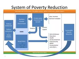
Factor markets Factor market functioning Segmentation Wage determination What do we want to capture? Macroeconomic Environment • Structural features • Binding macro constraints • General Equilibrium effects • Heterogeneity • Human and physical capital • Demographic Composition • Preferences • Access to Markets Households
Possible applications • Impact of macroeconomic shocks or policies on income distribution and poverty: • structural adjustment, • terms of trade, • devaluation, • fiscal reforms • Impact of poverty reduction policies: • food subsidies • schooling subsidies • public spending on health and/or education • public employment programs • Impact of demographic changes (demographic transition) on income distribution and poverty
What is a Microsimulation Model? • “The common denominators [of microsimulation models] are two, namely, that they all deal with behavior (decision) units at the micro (firm, household, etc.) levels and that they all aggregate up to large parts or all of the national economy.” Bergmann, Eliasson, and Orcutt, 1980. • “... instead of aggregating observations within a household survey into a few household groups in conformity with the requirements of CGE-type models, our aim should be to work directly with all the individual observations of the survey. By doing so, we hope to achieve full consistency between macroeconomic reasoning and standard poverty evaluation.” Bourguignon, 1999.
Elements for a typology • accounting vs. behavioral • reduced form vs. structural models • partial vs. general equilibrium • static vs. dynamic • sequential vs. integrated
4 types • Micro-accounting & disaggregated CGE models • Structure of income • Structure of consumption • Sequential approach & reduced form models • Reduced-form micro-econometric model of household income generation • Integrated approach & structural models • Structural specification of household decisions • Dynamic models
“Integrating Theory and Measurement” (Bergmann, Eliasson, and Orcutt, 1980) • Construction and validation of macroeconomic models • SAM production • CGE modeling • Development of microeconomic models of household behavior • Data base setting up • Events and behaviors modeling • Model Validation • Structural validity • specification of variables and relationships theoreticaly plausible? • initial parameters consistent with theory? • Operational validity : is the model able to answer the question raised ? • Empirical validity : are the base simulation results consistent with empirical observations ? • Micro-Macro modeling: macroeconomic model based on real microeconomic data • Reconciling household surveys and National Accounts data (Robilliard and Robinson, 2000)
Base and alternative simulations • Base Simulation : uses variables and parameters observed or most likely • Alternative simulations : • price changes (returns on labor market, devaluation, consumption prices, schooling costs, ...) • alternative policies, macroeconomic shocks • preferences changes (occupational choices, human capital investment, ….) • changes in socio-demographic characteristics (population ageing, migration, household structure changes, …)
Analyzing results • Growth : household income evolution (by socio-economic group) • Poverty : poverty rates (incidence, severity, inequlity among the poor, poverty profile) • Inequality : Lorenz Curves, Gini coefficient, Atkinson indices, entropie measures • Other indicators : schooling, health, migration, nutrition…..
Econometrics as a tool for building microsimulation models Example : modeling household income • occupational choices • wage and profit equations • non observable heterogeneity (individual fixed effects) • aggregation of income sources within each household
Occupational Choices • Selection of the population « at risk » • Binary choice: activity vs. inactivity --> probit, logit • Multiple choice : inactivity, wage work, agricultural self employment, non agricultural self employment --> multivariateprobit, multinomial logit • Ex. Multinomial Logit Individual i utility associated with activity j can be written: If agent i chooses j, then:
Occupational Choices • Assumption on the terms of error: the are independent and identically distributed according to a Weibull distribution • The probability that agent i chooses activity j, can be written : • The multinomiallogit implicitly assumes that irrelevant alternatives are independent (IIA). This means that agent i’s choice will remain unchanged if one of the irrelevant alternatives is modified. • STATA procedure: « mlogit »
Wage and profit equations • How does the labor market function? Segmentation or perfect integration? One income function or many sectoral ones? • Choice of the dependant variable? Average wage? Last month wage? How to distinguish profit and turnover in the agricultural sector? With or without family workers payment? • Mincer-type wage equation with log individual earnings regressed on years of schooling and years of work experience and its square
Wage and profit equations • Profit function with z : family work ; x : head’s education and experience • Family work might be endogenous • Exogeneity test, if rejected then • instrument, which means find variables that determine the quantity of travail, but are independent from profit (for instance, household composition) STATA procedure: « ivreg »
Non Observable Heterogeneity - taking into account the residual • Observables can only explain part of the variance of wages or profit • Omitting the residual (the unexplained part of the variance) is equivalent to omitting part of the variance and hence part of the inequality between individuals • If the residual is negative (positive) the agent is less (better) paid than the average of wage workers presenting identical characteristics • How can we model that residual ?
The Indonesia Model Bourguignon, Robilliard and Robinson (2002)
Background • The social impact of the financial crisis that hit Indonesia in 1997 has been the subject of ongoing research. • Recent data analyses suggest that the shock, while not as bad as once predicted, has led to important adjustments in labor markets (Manning, 2000) and an 66.8% increase in the poverty head-count ratio (Suryahadi et al., 2000) • The study attempts to quantify these adjustments and their effects on poverty and inequality.
MACRO Full Static Computable General Equilibrium Software: GAMS Data: Social Accounting Matrix for 1995 38 sectors 5 agricultural 15 informal 18 formal 15 factors of production 8 types of labor 7 types of capital marketing margins self consumption MICRO Reduced Form Occupational Choice Model Software: STATA Data: Savings-Investment module of SUSENAS 1996 9,800 households 33,400 individuals aged 10 years and older 8 labor segments 4 occupational choices at the individual level inactive wage worker self employed wage worker & self employed Characteristics of the sequential micro-macro model for Indonesia
The Sequential Framework Macro-level module (Extended CGE-type model) - Occupational structure: L - Price variables: p - Wage and earnings: w - All other variables in macro module: Y Link variables: L, w, p Micro-simulation module (Household survey) - Socio demographic characteristics: Si - Occupational/labor-supply choice: li = O(Si,) - Income: yi = E(Si,).li Consistency with macro. Find changes in parameters and such that: li = L and Mean E(Si,) = w Outcome = change in distribution of income conditionally on characteristics S.
Assume the CGE model will deliver where i is a segment, F indicates formal sectors (wage work), and I indicates informal sectors (self employment). • Let aki+ bk.zp + ukp be the utility for individual p of being in occupational group k (1 for wage work and 2 for self employment) where zp is a set of observed individual characteristics, ukp summarizes the effects of unobservables, aki is a constant, and bk is a vector of coefficients.
Let earning and profit functions write: where xpis a set of individual characteristics, m designates households, Zm is a set of household characteristics, Nm is the number of family workers, i, , and are sets of estimated coefficients, and are constants, and and vp summarize the effect of unobservables.
Let ( ) be the logical indicator function taking the value 1 if the expressions within brackets are true and zero otherwise. The problem can be written: find (a1i,a2i,i,)such that for all segments i.
Household incomes are then derived from the occupational choice functions and the earning and profit functions through: and OIm is non labor income (transfers, imputed rents,...etc).
Econometric Estimations • Earning functions for all segments: • Occupational choice model for heads, spouses and others: U0 = a0+ b0.zp + u0p inactivity work U1 = a1+ b1.zp + u1p wage work U2 = a2+ b2.zp + u2p self-employment U3 = a3+ b3.zp + u3p both • Profit functions for agricultural, informal and mixed activities:
Solution Algorithm Consider a set of nonlinear functions fi(P1,...,Pn), which yield the following problem: f(P) = 0 where P is the vector of variables and f is the vector of functions Any iteration procedure for solving this set of equations can be written as P(k+1) = P(k) + (k)d(k) where k refers to the iteration, d(k) is a direction vector, and (k) is a scalar giving the step of the size to be taken in direction d(k). In the Newton-Raphson procedure, the step size is equal to one and the direction vector writes: -D-1, where D is the matrix of derivatives of the functions P
Policy Analysis with CGE model simulations • Reproduce historical changes in occupational choices and real wages • Decompose historical change • Financial crisis • real devaluation • credit crunch • El Nino drough • Analyze alternative policy packages • targeted safety nets • food subsidy
Simulation Description SIMELN El Nino Drought SIMDEV Real Devaluation DEVCCF SIMDEV+ Foreign Credit Crunch FINCRI DEVCCF + Domestic Credit Crunch SIMALL FINCRI + El Nino Drought CGE Simulations: Decomposing the historical shock
Decomposing the social impact of the Indonesian financial crisis Notes: Base values for BASE column and percent change for other simulations. SIMELN El Niño Drought SIMDEV Real Devaluation DEVCCF Real devaluation + Foreign Credit Crunch FINCRI Real devaluation + Foreign Credit Crunch + Domestic Credit Crunch SIMALL Real devaluation + Foreign Credit Crunch + Domestic Credit Crunch + El Niño Drought Source: Robilliard, Bourguignon and Robinson 2001.
Real Devaluation + Foreign Credit Crunch + Domestic Credit Crunch + El Nino Drought% change in per capita income
Concluding Remarks • Overall changes in poverty are important and mainly fuelled by the negative income impact of the crisis. • Poverty indicators show that the impact is worse on the poorest of the poor. • Poverty rate increases in the urban sector are bigger than in the rural sector where inequality decreases. • Nevertheless, poverty indicators remain higher in the rural sector. • Increase of inequality in the urban sector is either offset by a decrease in the rural sector or by an decrease of inequality between the two sectors. • Socio-demographic changes play an important role in labor market changes and slightly offset the negative impact of the crisis in the rural sector.
Concluding Remarks (cont’d) • The CGE model does a relatively good job in reproducing changes in real wages and in occupational choices at aggregate level. • It does a less satisfactory job in reproducing changes in occupational choices by segment => more work on labor market specification and technology is needed. • The microsimulation module provides “reasonable” estimates of poverty and inequality changes. • It does not take fully into account socio-demographic changes.
The Madagascar Model Cogneau & Robilliard (2001)
Background • Declining GDP per capita since the beginning of the 70s. • Important contribution of the agricultural sector • 34% of GDP • 85% of active population • Failure of agricultural policies • low investment • bias against agriculture • low productivity • What development strategy for poverty reduction?
MACRO Stylized CGE Framework: endogenous prices for labor and goods markets Data: Social Accounting Matrix for 1995 3 goods 1 agricultural 1 informal 1 formal 5 factors of production 3 types of labor 2 types of capital MICRO Structural labor allocation model: Endogenous occupational choice and time allocation Data: Enquete Permanente aupres des Menages 1993 4,500 households 12,000 individuals aged 15 years and older 4 occupational choices at the household level farmer informal wage worker formal wage worker (rationed) farmer & wage worker Characteristics of the integrated micro-macro model for Madagascar • Software: GAUSS
The Integrated Framework Macro-level module (Extended CGE-type model) - Occupational structure: L - Price variables: p - Wage and earnings: w - All other variables in macro module: Y Micro-simulation module (Household survey) - Socio demographic characteristics: Si - Occupational/labor-supply choice: li = O(Si,E) - Income: yi = E(Si,w).li E = earning rate of individual/household i in various occupations. These “personal” rates are a function of a set of standard market rates, w. Outcome = change in distribution of income conditionally on characteristics S. Aggregating: li = L
Impact on poverty and income distribution of alternative development strategies in Madagascar Notes: Base values for BASE column and percent change for other simulations. EMBFOR Formal hiring (10 per cent) SALFOR Increase in formal wages (10 per cent) PGFAGRI Increase in total factor productivity in agricultural sector (10 per cent) PGFALIM Increase in total factor productivity in agricultural foodstuffs sector (10 per cent) Source: Cogneau and Robilliard 2001.
Conclusions • General equilibrium mechanisms have significant redistribution effects • The “lognormal-with-fixed-variance” assumption can yield biased results • In order to be effective in reducing poverty, any development strategy based on the growth of the urban/formal sector has to be redistributed to the agricultural/rural households through an improvement in the agricultural terms of trade
The Cote d’Ivoire Model Cogneau & Grimm (2002)