Download
1 / 47
470 likes | 499 Views
Explore how aerosols evolve in proximity to clouds & the impact of cloud effects on aerosol retrieval using satellite data. Investigate the growth of aerosols near clouds & the varied effects of cloud contamination and adjacency on aerosol optical properties. Learn about the interplay between aerosols, clouds, and radiative interactions in the atmosphere.

E N D
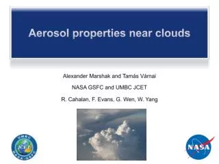
The apparent bluing of aerosols near clouds Alexander Marshak (GSFC) Guoyong Wen and Tamás Várnai (UMBC/GSFC) Lorraine Remer and Bob Cahalan (GSFC) Jim Coakley (OSU) and Norman Loeb (LRC)
Aerosols and Clouds1-km Terra MODIS Data 0.55-m Aerosol Optical Depth 0.86-m Fine Particle Fraction Fine Sun Glint Boundary Mixed Coarse Alexander Marshak Courtesy of Jim Coakley
MODIS Aerosol Optical Depthand Cloud Cover Sun Glint Boundary • Aerosols grow in humid environments near • clouds. • Aerosols grow through in-cloud processing. • Aerosols remain when droplets evaporate • New particle production in the vicinity of • clouds. • Illumination of cloud-free columns enhanced • through scattering of sunlight by nearby • clouds. • Cloud contamination of the cloud-free pixels • used to obtain aerosol properties. • Aerosols are precursors to cloud formation. Courtesy of Jim Coakley Alexander Marshak
What happens to aerosol in the vicinity of clouds? All observations show that aerosols seem to grow near clouds or (to be safer) “most satellite observations show a positive correlation between retrieved AOT and cloud cover”, e.g.: Cloud Fraction (%) from Ignatov et al., 2005 from Loeb and Manalo-Smith, 2005 from Zhang et al., 2005 Alexander Marshak
What happens to aerosol in the vicinity of clouds? All observations show that aerosols seem to grow near clouds. However, it is not clear yet how much grows comes from • “real” microphysics, e.g. • increased hydroscopic aerosol particles, • new particle production or • other in-cloud processes. • (“artificial”) the 3D cloud effects in the retrievals: • cloud contamination, • extra illumination from clouds Alexander Marshak
How do clouds affect aerosol retrieval? • clouds are complex and “satellite analysis may be affected by potential cloud artifacts” (Kaufman and Koren, 2006); • Both • cloud contamination (sub-pixel clouds) • cloud adjacency effect (a clear pixel with in the vicinity of clouds) • may significantly overestimate AOT. • But they have different effects on the retrieved AOT: while cloud contamination increases “coarse” mode, cloud adjacency effect increases “fine” mode. Alexander Marshak
The Ångström exponent and the cloud fraction vs. AOT • Atlantic ocean, June-Aug. 2002; each point is aver. on 50 daily values with similar AOT in 1o res.; • for AOT < 0.3, as AOT increases CF and the Ångström exponent also increase; • the increase is due totransition from pure marine aerosol to smoke (or pollution); • the increase in AOT cannot be explained by cloud contamination but rather aerosol growth. from Kaufman et al., IEEE 2005 Alexander Marshak
More clouds go with larger AOT and larger (not smaller!) Ångström exponent • 25 1ox1o in each 5ox5o region over ocean (off the cost of Africa) are subdivided into two groups with • a <a> • and • a <a> • meteorology has been checked as similar for two groups Courtesy of Norman Loeb (A-train presentation, Lille Oct. 2007) Alexander Marshak
More clouds go with larger AOT and larger (not smaller!) Ångström exponent • 25 1ox1o in each 5ox5o region over ocean (over the entire globe) are subdivided into two groups with • a <a> • and • a <a> • meteorology has been checked as similar for two groups Difference in cloud fraction Difference in fine-mode fraction Courtesy of Norman Loeb (A-train presentation, Lille Oct. 2007) Alexander Marshak
AOT and Ångström exponent vs. distance from the nearest cloud (AERONET data) Ångström exponent AOT (0.47 m) The Ångström exponent increases with distance to the nearest cloud while the AOT increases Time passed from the last cloud (min) from Koren et al., GRL, 2007 Alexander Marshak
3D ? Enhancement of radiance near cloudsCumulus clouds over Atlantic at 0.87 m 20 1000x500 km scenes analyzed from Koren et al., GRL, 2007 Alexander Marshak
Airborne aerosol observations in the vicinity of clouds From airborne extinction rather than scattering observations 3D effects decrease AOT rather than increase it Alexander Marshak Courtesy of Jens Redemann
cloudy clear (Chiu et al., 2008, in preparation) ARM Shortwave Spectrometertransition between cloudy and clear skies • two Cu clouds during the first and last 5 to 8 sec. • clear sky is evident about 15 sec. away from these periods; • the measurements in the intervening period (5 to 12 s and 75 to 82 s) are difficult to classify; • depending on the remote sensing criterion used for cloud detection, would be called either cloudy or clear. measurements of P. Pilewskie
c 5 Distance (km) 5 A simple 3D RT experiment cloudy 0.3 km clear 5 km 5 km 0 Alexander Marshak
A simple 3D RT experiment Courtesy of Toby Zinner vegetated surface black surface 0 Alexander Marshak
Aerosol-cloud radiative interaction (a case study) Collocated MODIS and ASTER image of Cu cloud field in biomass-burning region in Brazil at 53o W on the equator, acquired on Jan 25, 2003 Wen et al., 2006
Thin clouds Thick clouds ASTER image and MODIS AOT ASTER image MODIS AOT from Wen et al., JGR, 2007 Alexander Marshak
A striking example: const AOT Modeled (with const AOT but MODIS 3D cloud structure) vs Observed Reflectance. Cor. coef. = 0.77 Alexander Marshak
D~ 0.0046 D~0.05 ≈50% D~ 0.014 D~0.14 ≈140% Cloud effect at 90-m resolution Thick clouds, <>=14 Thin clouds, <>=7 AOT0.66=0.1 enhancement: D 3D-1D Alexander Marshak
Effect of distance to a cloudy pixel 3D enhancement (red) Cumulative distr. (blue) 0.66 m Nearest cloud dist. (km) Alexander Marshak
Conceptual model to account for the cloud-induced enhancement MODIS sensor molecule + aerosol aerosol or molecule Alexander Marshak surface
3D cloud enhancement For dark surfaces and aerosols below the cloud tops,the enhancement only weakly depends on the AOT Contributors to cloud enhancement enhancement: D 3D-1D • Rayleigh scattering • Aerosols • Surface reflectance AOT=0.1 AOT=0.5 AOT=1.0 Surface albedo Alexander Marshak
Conceptual model to account for the cloud enhancement (at 0.47 m) MODIS sensor from Wen et al., JGR 2008: molecule (82%) + aerosol (15%) aerosol or molecule Alexander Marshak surface (3%)
Assumption for a simple model Molecular scattering is the main source for the enhancement in the vicinity of clouds thus we retrieve larger AOT and fine mode fraction Alexander Marshak
Rayleigh layer Broken cloud layer How to account for the 3D cloud effect on aerosols? • The enhancement is defined as the difference between the two radiances: • one is reflected from a broken cloud field with the scattering Rayleigh layer above it • and one is reflected from the same broken cloud field but with the Rayleigh layer having extinction but no scattering Alexander Marshak from Marshak et al., JGR, 2008
Stochastic model of a broken cloud field • Clouds follow the Poisson distr. and are defined by • average optical depth, <> • cloud fraction, Ac • aspect ratio, AR = hor./vert. AR = 2 AR = 1 Ac = 0.3 Alexander Marshak
Stochastic model of a broken cloud field • Clouds follow the Poisson distr. and are defined by • average optical depth, <> • cloud fraction, Ac • aspect ratio, AR = hor./vert. AR = 2 AR = 1 Ac = 0.3 Alexander Marshak
Cloud-induced enhancement at 0.47 m LUT: The enhancement vs <> for AR = 1. Ac=1 corresponds to the pp approximation. Alexander Marshak
Cloud-induced enhancement:our simple model and 3D RT calculations The enhancement vs <> for Ac= 0.6 and 3 cloud AR = 0.5, 1 and 2. Different dots are from Wen et al. (2007) MC calculations for the thin and thick clouds. Alexander Marshak
Ångström exponent Ångström exponent vs <> for Ac= 0.5 and AR = 2. Three cases: clean, polluted and very polluted. very polluted very polluted 0.47 m vs. 0.65 m 0.65 m vs. 0.84 m polluted polluted clean clean The cloud adjacency effect increases the Ångström exponent Alexander Marshak
MODIS observations(Várnai and Marshak, 2008, in preparation) • Collection 5 MOD02, MOD06, MOD35 products • September 14-29 in 2000-2006 (2 weeks in 7 years) • North-East Atlantic (45°-50°N, 5°-25°W), south-west from UK • Viewing zenith angle < 10° • Pixels included in plots: • Ocean surface with no glint or sea ice • MOD35 says “confident clear”, all 250 m subpixels clear • Highest cloud top pressure nearby > 700 hPa (near low clouds) • Nearby pixels are considered cloudy if MOD35 says definitely cloud.
Average reflectance vs. dist. to clouds for 0.45, 0.65, 0.87, 2.1 and 11 m mean and std
Reflect. Dist to Clouds vs Cloud Optical Depth 0.47 m # of pixels log of # of pixels Dist. to cloud (km)
Reflect. Diff from Values at 10 km vs Cloud Optical Depth 2.10 m
Reflect. Diff from Values at 10 km vs Cloud Optical Depth 0.87 m
Reflect. Diff from Values at 10 km vs Cloud Optical Depth 0.65 m
Reflect. Diff from Values at 10 km vs Cloud Optical Depth 0.47 m
Cloud enhancement vs. dist. to clouds for 0.45, 0.65, 0.87, and 2.1 m
Point spread function effect for 0.53 m(preliminary results) with Jack Xiong
Cloud contamination in 0.47 m(preliminary results) • latency effect removed (red curve); • assumed that at 2.1 m the increase is due to undetected subpixel clouds (blue curve) • assumed that 2.1 m has the same point spread function as 0.53 m (green curve) with Jack Xiong
with Norman Loeb and Lorraine Remer Work in progress • select a few MODIS subscenes with • broken low Cu; • retrieved AOT; • over ocean with no glint, etc; • analyze AOT, CF, average COD over many 10 x 10 km areas; • use a simple stochastic model and RT to estimate upward flux; • use CERES fluxes to convert BB to spectral fluxes; • use ADM to determine spectral fluxes from MODIS radiances; • estimate cloud enhancement and compare the results; • use a simple linearization model.
with Ralph Kahn, Jens Redemann and Phil Russell Work in progress • The NASA ARCTAS aircraft mission will take place in spring/summer 2008. • Cloud-scattered Light Experiment • To characterize the cloud-scattered light field to interpret satellite radiance observ. in the “halo” region surrounding clouds. • Using SSFR to measure up- and down-welling spectral radiative flux as a function of • distance to (water) cloud • COD, cloud base, cloud height, AR • vertical distribution of aerosols • surface spectral albedo • etc. • Below cloud and well-above cloud with • multiple horizontal distances from cloud
Conclusions • No clear understanding from satellites alone of what happens to aerosols at the vicinity of clouds. (The twilight zone?) • Accounting for the 3D cloud-induced enhancement helps. • For certain conditions, 3D cloud enhancement • 3D1D • only weakly depends on AOT and molecular scatt. is the key source for the enhancement. • The enhancement increases the “apparent” fraction of fine aerosol mode (“bluing of the aerosols”). • MODIS observations confirm that the cloud induced enhancement increases with cloud optical depth. • Retrieved AOT can be corrected for the 3D radiative effects. Alexander Marshak
point spread function and latency effect removed (blue curve); • assumed that at 2.1 m the increase is due to undetected subpixel clouds (green curve) • assumed that 2.1 m has the same point spread function as 0.53 m (black curve) Point spread function effect for 0.53 m(preliminary results) with Jack Xiong
Cloud enhancement vs. cloud reflectance The upwelling flux is needed to estimate the cloud-induced enhancement of cloud-free pixels Alexander Marshak