Download
1 / 50
500 likes | 601 Views
Explore the intricate details of vibrational motion in pump-probe experiments with iodine ions, revealing insights into electronically excited intermediate states and their coupling to final states. Gain knowledge about ionization, potential curves, and dynamics impacting strong-field physics and quantum tomography.

E N D
Strong-field physics revealed through time-domain spectroscopy George N. Gibson University of Connecticut Department of Physics Grad student: Li Fang Funding: NSF-AMO May 30, 2009 XI Cross Border Workshop on Laser Science University of Ottawa, Ottawa, Canada
Motivation • Vibrational motion in pump-probe experiments reveals the role of electronically excited intermediate states. • This raises questions about how the intermediate states are populated. Also, we can study how they couple to the final states that we detect. • We observe inner-orbital ionization, which has important consequences for HHG and quantum tomography of molecular orbitals.
Pump-probe experiment with fixed wavelengths. In these experiments we used a standard Ti:Sapphire laser: 800 nm 23 fs pulse duration 1 kHz rep. rate Probe Pump
Pump-probe spectroscopy on I22+ Enhanced Excitation Enhanced Ionization at Rc Internuclear separation of dissociating molecule
Vibrational structure Depends on: • wavelength (400 to 800 nm). • relative intensity of pump and probe. • polarization of pump and probe. • dissociation channel. • We learn something different from each signal. • Will try to cover several examples of vibrational excitation.
(2,0) vibrational signal • Amplitude of vibrations so large that we can measure changes in KER, besides the signal strength. • Know final state – want to identify intermediate state.
Simulation results From simulations: - Vibrational period- Wavepacket structure- (2,0) state
What about the dynamics? • How is the A-state populated? • I2 I2+ (I2+)* - resonant excitation? • I2 (I2+)* directly – innershell ionization? • No resonant transition from X to A state in I2+.
From polarization studies • The A state is only produced with the field perpendicular to the molecular axis. This is opposite to most other examples of strong field ionization in molecules. • The A state only ionizes to the (2,0) state!?Usually, there is a branching ratio between the (1,1) and (2,0) states, but what is the orbital structure of (2,0)? • Ionization of A to (2,0) stronger with parallel polarization.
Implications for HHG and QT • We can readily see ionization from orbitals besides the HOMO. • Admixture of HOMO-1 depends on angle. • Could be a major problem for quantum tomography, although this could explain some anomalous results.
(2,0) potential curve retrieval It appears that I22+ has a truly bound potential well, as opposed to the quasi-bound ground state curves. This is an excimer-like system – bound in the excited state, dissociating in the ground state. Perhaps, we can form a UV laser out of this.
Wavelength-dependent pump probe scheme • Change inner and outer turning points of the wave packet by tuning the coupling wavelength. • Femtosecond laser pulses: Pump pulse: variable wavelength. (517 nm, 560 nm and 600 nm.) Probe pulse: 800 nm.
Vibrational period (fs) X-B coupling wavelength (nm) I2+ spectrum: vibrations in signal strength and kinetic energy release (KER) for different pump pulse wavelength [517nm, 560 nm and 600 nm]
pump-probe delay=180 fs Simulation: trapped population in the (2,0) potential well The (2,0) potential curve measured from the A state of I2+ in our previous work: PRA 73, 023418 (2006)
Neutral ground state vibrations in I2 • Oscillations in the data appear to come from the X state of neutral I2. • Measured the vibrational frequency and the revival time.
Revival structure • Vibrational frequencyMeasured 211.00.7 cm-1Known 215.1 cm-1Finite temp 210.3 cm-1
Raman scattering/Bond softening • Raman transitions are made possible through coupling to an excited electronic state. This coupling also gives rise to bond softening, which is well known to occur in H2+.
Lochfrass • New mechanism for vibrational excitation: “Lochfrass”R-dependent ionization distorts the ground state wavefunction creating vibrational motion. • Seen by Ergler et al. PRL 97, 103004 (2006) in D2+.
Lochfrass vs. Bond softening • Can distinguish these two effects through the phase of the signal. • LF = • BS = /2.
Iodine vs. Deuterium • Iodine better resolved: 23 fs pulse/155 fs period = 0.15 (iodine) 7 fs pulse/11 fs period = 0.64 (deuterium) • Iodine signal huge: • DS/Save = 0.60 • DS/Save = 0.10
Variations in kinetic energy • Amplitude of the motions is so large we can see variations in KER or <R>.
Temperature effects • Deuterium vibrationally cold at room temperatureIodine vibrationally hot at room temperature • Coherent control is supposed to get worse at high temperatures!!! But, we see a huge effect. Intensity dependence also unusual • We fit <R> = DRcos(wt+j) +RaveAs intensity increases, DR increases, Rave decreases.
Intensity dependence • Also, for Lochfrass signal strength should decrease with increasing intensity, as is seen.
But, Rave temperature: T decreases while DR increases!!!
We have an incoherent sea of thermally populated vibrational states in which we ionize a coherent hole: • So, we need a density matrix approach.
Density matrix for a 2-level model • For a thermal system where p1(T) and p2(T) are the Boltzmann factors. This cannot be written as a superposition of state vectors.
Time evolution of r • We can write: • These we can evolve in time.
Coherent interaction – use p/2 pulse for maximum coherence • Off diagonal terms have opposite phases. This means that as the temperature increases, p1 and p2 will tend to cancel out and the coherence will decrease.
R-dependent ionization – assume only the right well ionizes. • yf = (yg + ye)/2 • Trace(r) = ½ due to ionization What about excited state? NO TEMPERATUREDEPENDENCE!
Expectation value of R, <R> The expectation values are p/2 out of phase for the two interactions as expected.
Coherent interactions: Off diagonal terms are imaginary. Off diagonal terms of upper and lower states have opposite signs and tend to cancel out. R-dependent ionization Off-diagonal terms are real. No sign change, so population in the upper state not a problem. Comparison of two interactions Motion produced by coherent interactions and Lochfrass are p/2 out of phase.
“Real” (many level) molecular system • Include electronic coupling to excited state. • Use I(R) based on ADK rates. Probably not a good approximation but it gives R dependence. • Include n = 0 - 14
Same conclusions For bond-softening • Off-diagonal terms are imaginary and opposite in sign to next higher state. r12(1) -r12(2) • DR decreases and <n> increases with temperature. For Lochfrass • Off diagonal terms are real and have the same sign. r12(1)r12(2) • DR increases and <n> decreases with temperature.
Excitation from Lochfrass will always yield real off diagonal elements with the same sign for excitation and deexcitation [f(R) is the survival probablility]:
Conclusions Coherent reversible interactions • Off-diagonal elements are imaginary • Excitation from one state to another is out-of-phase with the reverse process leading to a loss of coherence at high temperature • Cooling not possible Irreversible dissipative interactions • Off-diagonal elements are real • Excitation and de-excitation are in phase leading to enhanced coherence at high temperature • Cooling is possible
Conclusions • Excitation of the A-state of I2+ through inner-orbital ionization • Excitation of the B-state of I2 to populate the bound region of (2,0) state of I22+ • Vibrational excitation through tunneling ionization.
Laser System • Ti:Sapphire 800 nm Oscillator • Multipass Amplifier • 750 J pulses @ 1 KHz • Transform Limited, 25 fs pulses • Can double to 400 nm • Have a pump-probe setup