Download
1 / 37
370 likes | 516 Views
The equations of motion and their numerical solutions III. by Nils Wedi (2006) contributions by Mike Cullen and Piotr Smolarkiewicz. Boundaries.

E N D
The equations of motion and their numerical solutions III by Nils Wedi (2006) contributions by Mike Cullen and Piotr Smolarkiewicz
Boundaries • We are used to assuming a particular boundary that fits the analytical or numerical framework but not necessarily physical free surface, non-reflecting boundary, etc. • Often the chosen numerical framework favors a particular boundary condition where its influence on the solution remains unclear
Choice of vertical coordinate • Ocean modellers claim that only isopycnic/isentropic frameworks maintain dynamic structures over many (life-)cycles ? .. Because coordinates are not subject to truncation errors in ordinary frameworks. • There is a believe that terrain following coordinate transformations are problematic in higher resolution due to apparent effects of error spreading into regions far away from the boundary in particular PV distortion. However, in most cases problems could be traced back to implementation issues which are more demanding and possibly less robust to alterations. • Note, that in higher resolutions the PV concept may loose some of its virtues since the fields are not smooth anymore, isentropes overturn and cross the surface.
Choice of vertical coordinate • Hybridization or layering needed to exploit the strength of various coordinates in different regions (in particular boundary regions) of the model domain • Unstructured meshes: CFD applications typically model only simple fluids in complex geometry, in contrast atmospheric flows are complicated fluid flows in relatively simple geometry (eg. gravity wave breaking at high altitude, trapped waves, shear flows etc.) Bacon et Al. (2000)
But why making the equations more difficult ? • Choice: Use relatively simple equations with difficult boundaries or use complicated equations with simple boundaries • The latter exploits the beauty of “A metric structure determined by data” Freudenthal, Dictionary of Scientific Biography (Riemann), C.C. Gillispie, Scribner & Sons New York (1970-1980)
Examples of vertical boundary simplifications • Radiative boundaries can also be difficult to implement, simple is perhaps relative • Absorbing layers are easy to implement but their effect has to be evaluated/tuned for each problem at hand
Radiative Boundary Conditions for limited height models eg.Klemp and Durran (1983); Bougeault (1983); Givoli (1991); Herzog (1995); Durran (1999) Linearized Boussinesq Equations in x-z plane
Radiative Boundary Conditions Inserting… Dispersion relation: Phase speed: for hydrostatic waves Group velocity:
Radiative Boundary Conditions discretized Fourier series coefficients:
Wave-absorbing layers eg. Durran (1999) Adding r.h.s. terms of the form … Viscous damping: Rayleigh damping:
Flow past Scandinavia 60h forecast 17/03/1998 divergence patterns in the operational configuration
Flow past Scandinavia 60h forecast 17/03/1998divergence patterns with no absorbers aloft
Wave-absorbing layers: overlapping absorber regions Finite difference example of an implicit absorber treatment including overlapping regions
The second choice … • Create a unified framework to investigate the influence of upper boundary conditions on atmospheric and oceanic flows • Observational evidence of time-dependent well-marked surfaces, characterized by strong vertical gradients, ‘interfacing’ stratified flows with well-mixed layers Can we use the knowledge of the time evolution of the interface ?
Generalized coordinate equations Strong conservation formulation !
Explanations … Using: Jacobian of the transformation Transformation coefficients Contravariant velocity Solenoidal velocity Physical velocity
Time-dependent curvilinear boundaries • Extending Gal-Chen and Somerville terrain-following coordinate transformation ontime-dependent curvilinear boundaries Wedi and Smolarkiewicz (2004)
Swinging membrane Animation: Swinging membranes bounding a homogeneous Boussinesq fluid
Another practical example • Incorporate an approximate free-surface boundary into non-hydrostatic ocean models • “Single layer” simulation with an auxiliary boundary model given by the solution of the shallow water equations • Comparison to a “two-layer” simulation with density discontinuity 1/1000
Regime diagram supercritical Critical, downstream propagating lee jump critical, stationary lee jump subcritical
Critical – reduced domain flat shallow water
Conclusions • …collapses the relationship between auxiliary boundary models and the interior fluid domain to a single variable • …aids the systematic investigation of influences of different boundary conditions on the same flow simulation • …possibly simplifies the direct incorporation of observational data into flow simulations given the exact knowledge of H and it’s derivative • Aids the inclusion of a free surface in ocean data assimilation and corresponding adjoint formulation
The stratospheric QBO • westward • + eastward data taken from ERA40
Laboratory analogue of the quasi-biennial oscillation (QBO) • The coordinate transformation allows for a time-dependent upper/lower boundary forcing without small amplitude approximation • Demonstrates the importance of wave transience and their correct numerical realization when resulting in a dominant large scale oscillation
The laboratory experiment of Plumb and McEwan • The principal mechanism of the QBO was demonstrated in the laboratory • University of Kyoto Plumb and McEwan, J. Atmos. Sci. 35 1827-1839 (1978) http://www.gfd-dennou.org/library/ gfd_exp/exp_e/index.htm Animation:
Time – height cross section of the mean flow Uin a 3D simulation Animation Wedi and Smolarkiewicz, J. Atmos. Sci., 2006 (accepted)
Viscous simulation Eulerian semi-Lagrangian Wedi, Int. J. Numer. Meth. Fluids, 2006
Inviscid simulation Eulerian St=0.36, n=640 Eulerian St=0.25, n=384 semi-Lagrangian St=0.25, n=384 top rigid, freeslip top rigid, freeslip top absorber
Conclusions • The flux-form Eulerian simulation is asymptotically close to “idealized inviscid”. • The semi-Lagrangian simulation exhibits a more viscous behaviour due to enhanced dissipation, which contributes to the development of different bifurcation points in the flow evolution. • The analysis is relevant to larger-scale geophysical flows driven by small scale fluctuations, where the interplay of reversible and irreversible fluxes determines the flow evolution.
Numerically generated forcing ! Instantaneous horizontal velocity divergence at ~100hPa No convection parameterization Tiedke massflux scheme T63 L91 IFS simulation over 4 years Interaction of convection (parametrization) and the large-scale dynamics appears to play a key role in future advances of forecast ability!