Download
1 / 48
480 likes | 547 Views
Explore the study of high-pressure systems and turbulent mixing in high-energy-density physics using lasers and shock waves. Follow experiments, implications, and theoretical considerations in this comprehensive guide backed by research grants.

E N D
Approaches to Turbulence in High-Energy-Density Experiments R. Paul Drake University of Michigan 2007 TMBW, Trieste Work supported by the U.S. Department of Energy under grants DE-FG52-07NA28058, DE-FG52-04NA00064, by the Naval Research Laboratory under contract NRL N00173-06-1-G906, and by othergrants and contracts
Who contributed; where we are going • Key collaborators (others listed later) • Michigan: C.C. Kuranz, E.C. Harding, M. Grosskopf • LLNL: J.F. Hansen, H.F. Robey, B.A. Remington, A. Miles • Rochester: J. Knauer • Florida State: T. Plewa • NRL: Yefim Aglitskiy • Outline • How lasers accomplish hydrodynamic experiments • Shock-driven Richtmyer Meshkov • Turbulence? • Blast-wave-driven instabilities & why not yet turbulent • Steepness of shear appears to matter (blast-waves, jets) • An experiment to create a steep shear layer • An experiment having a steep shear layer and turbulence • Some speculation regarding requirements for quick turbulence Turbulent Mixing and Beyond
High-Energy-Density Physics • The study of systems in which the pressure exceeds 1 Mbar (= 0.1 Tpascal = 1012 dynes/cm2), and of the methods by which such systems are produced. • This also matters for astrophysics • Direct reasons • pressures > 1 Mbar are important in planets • High-temperature dense matter is important in stars • Indirect reasons • Dynamics of Mach >> 2, very high Re systems • T >> 1 eV (104 K) and/or = (8p/B2) >> 1 systems • Radiation hydrodynamic systems • We work in my group with high Mach number hydrodynamic and radiative hydrodynamic systems Turbulent Mixing and Beyond
The Omega laser is our major tool at present Omega is at the Laboratory for Laser Energetics, affiliated with the University of Rochester. Its primary mission is inertial fusion research. Target chamber at Omega laser There are lots of kJ, ns lasers around the world Omega is the most capable for experiments. Turbulent Mixing and Beyond
Here is what such lasers do to a material • The laser is absorbed at less than 1% of solid density Rad xport, high-v plas Hydro, rad hydro From Drake, High-Energy-Density Physics, Springer (2006) Turbulent Mixing and Beyond
Shock waves establish the regime of an experiment Turbulent Mixing and Beyond
The Mach number in these experiments is effectively infinite • Sound speeds are ~ 1 km/sec • Exact value depends on upstream “preheating” • Shock velocities are ~ 50 km/sec • Mach number terms in shock jump relations are fundamentally present as 1/M2 • Implications • Density jump is ~ (– 1)/(– 1) • Post-shock temperature is ~ • Here , Z are post-shock values • A complication is that they are temperature-dependent. Turbulent Mixing and Beyond
Here is a drawing of a typical target for hydrodynamics experiments on lasers • Precision structure inside a shock tube Experiment design: Carolyn Kuranz Turbulent Mixing and Beyond
Ungated imaging provides improved resolution in such experiments (side-on schematic) Drive beams t=0 20 mm Au shield protects film from overexposure 4 backlighter beams X-ray photons Delayed 10-30 ns Target Titanium/Scandium backlit pinhole X-ray film Turbulent Mixing and Beyond Credit: Carolyn Kuranz
This shows images of actual targets built at Michigan Side view Laser-driven surface Acrylic cone Gold cone 1 mm Targets: Mike Grosskopf, Donna Marion, Robb Gillespie, UROP team Turbulent Mixing and Beyond
Alignment in Omega Chamber XTVS YTVS Turbulent Mixing and Beyond
What a shot looks like in the chamber… Backlighter positioner Backlighter stalk Main target positioner Acrylic shield Turbulent Mixing and Beyond
We have greatly improved the resolution and signal-to-noise in the data Aug. 2005 Dec. 2006 Grid squares have 43 µm openings Eggcrate mode only, 20 to 50 µm stepped pinhole, 17 ns Eggcrate + 424 µm sine wave, 10 to 20 µm tapered pinhole, 25 ns Mid-1990’s data Also, the UM-led team was the first group to get simultaneous orthogonal physics data Recent data and analysis: Carolyn Kuranz Turbulent Mixing and Beyond
Theoretical considerations for these experiments • One likes to imagine that these systems are described by the Euler equations • But do these accurately describe the physical system? r = density v = velocity p = pressure g = constant (adiabatic index) Turbulent Mixing and Beyond
Is it sufficient to use only hydrodynamics? • General Fluid Energy Equation: Material Energy Flux m Smaller or Hydro-like Typ. small Or Ideal MHD Turbulent Mixing and Beyond
Typical parameters in these experiments • U ~ 10 km/s Range 1 to < 1,000 • Driving scale for turbulence ~ 100 µm Range 10 µm to 1 mm • Kinematic viscosity ~ 10-5 m2/s Range 10-6 to 10-4 • Re ~ 105 Range 104 to 107 • Kolmogorov scale ~ 0.02 µm • Viscosity ~ Diffusion (Schmidt # ~1). RT & RM typically quenched on scales of 1 to a few µm (Robey 2004) • Pe and Perad are both >>> 1 • The plasmas are well localized (fluid models are OK) See: D.D. Ryutov, et al. ApJ 518, 821 (1999); ApJ Suppl. 127, 465 (2000); Phys. Plasmas 8, 1804 (2001) Turbulent Mixing and Beyond
Consider what we mean by “turbulence” • Is turbulence • Growth of structures beyond the nonlinear saturation of existing modes? • The development of strong mixing as indicated by supra-linear growth of a mixing layer in time? • The appearance of an inertial range in the fluctuation spectrum? • Something else? • Different communities use different definitions • For turbulence corresponding to strong mixing • Dimotakis (2000) argued that the necessary condition was a sufficient separation of the Taylor microscale and the dissipation scale Turbulent Mixing and Beyond
Does the large Re lead to “turbulence”? • HEDP experiments typically have Re of 104 to 106 The Dimotakis picture. Credit: Zhou 2003 Turbulent Mixing and Beyond
The experimental Re is > 105, so these systems should be turbulent? • Let’s look at Richtmyer-Meshkov • Practical experiments are “heavy to light” From Drake, High-Energy-Density Physics, Springer (2006) Turbulent Mixing and Beyond
At high Mach number, RM does not become turbulent by almost any definition • Hard experiments • Difficult to sustain the shock • Glendinning et al. (Phys. Plas., 2003) • The spikes rapidly overtake the shock, distorting it and limiting their development • Initial amplitude 5% • Sensible result: • Incompressible Meyer-Blewett amplitude growth (d/dt) • Can exceed the shock separation velocity data simulation Turbulent Mixing and Beyond
Do we see turbulence in scaled hydrodynamic experiments relevant to supernovae? • SN 1987A • A core-collapse supernova • Early high-Z x-ray lines with large Doppler shifts • Early glow from radioactive heating • The issue is the post-core-collapse explosive behavior • In 19 years of simulations • Only one (Kifonidis, 2006) makes fast enough high-Z material • 3D simulations coupling all the interfaces where initial conditions matter are not feasible • Experiments will be able to address this fully within a decade • We now address a single interface SN1987A, WFPC2, Hubble Kifonidis, 2003 Turbulent Mixing and Beyond
This type of system involves a blast-wave-driven interface • Laser ablation drives shock wave for 1 ns • Front surface rarefaction overtakes shock wave by 2 ns, forming planar blast wave • Blast wave crosses interface, followed by deceleration and rarefaction From Drake, High-Energy-Density Physics, Springer (2006) Turbulent Mixing and Beyond
Boundary conditions in time & space matter for scaling Pressure and density Interface velocity vs time star lab Conclusion: scaling is possible Turbulent Mixing and Beyond
There is a turbulence angle to these experiments and supernovae Kifonidis et al., 2003 Van Dyke, Album of Fluid Motion All simulations have too much numerical viscosity to produce the observed turbulent state. But it is an open question whether the flows in supernovae actually become turbulent Kelvin-Helmholtz roll-up Laminar flow Experimental image of aturbulent flow at Re = 3x10⁴ Numerical image of an unstable, though non-turbulent flow at Re(sim) ~ 103; Re = 1010 Turbulent Mixing and Beyond
shock shock shock Our Rayleigh-Taylor experiments produce time-dependent, high-Reynolds-number systems. bubbles spikes t = 8 ns t = 12 ns t = 14 ns • Data from a 2D single-mode perturbation having an initial perturbation l0 = 50 µm, a0 = 2.5 µm, ka0 = 0.3 •The perturbation growth is well into the non-linear regime and Re > 3 x 104 by 7 ns, but the system does not appear to become turbulent within 14 (or 20) ns Turbulent Mixing and Beyond
The question is why these experiments did not enter a turbulent state • One answer is time dependence • For turbulence corresponding to strong mixing • Dimotakis (2000) argued that the necessary condition was a sufficient separation of the Taylor microscale and the dissipation scale • Zhou et al. (2003) and Robey et al. (2003) argued that sufficient time was also needed • The role of large Re is to allow diffusive laminar boundary layers to become large enough to separate driving scales from dissipation scales • This also takes time • Miles et al. (2004, 2005) argued from simulations that interacting structures could produce turbulent conditions, but not soon enough to be observed in the Omega experiments Turbulent Mixing and Beyond
Here is the Robey/Zhou picture • The point is • It can take longer to establish the needed boundary layers than it does to reach the threshold value of Re • Zhou et al. 2003 show that this picture applies successfully to numerous cases The Robey/Zhou picture. Credit: Robey 2003 Turbulent Mixing and Beyond
This picture is consistent but not universal • Consistency: • Dimotakis requires that the Liepmann-Taylor scale exceed the inner viscous scale, or 5Re-1/2 > 50Re-3/4 • Robey/Zhou requires the viscous boundary layer, 5(t)1/2 > 50Re-3/4 • These are consistent if t = /U • For typical turbulence /U = l/u, a large-eddy turnover time, so both these arguments are consistent with development of an inertial range and strong mixing in one eddy turnover time • I will refer to this as “quick turbulence”, distinct from e.g. long-term RT • Issues • Perhaps /U ≠ l/u. • Sometimes velocity shear is gentle … Turbulent Mixing and Beyond
The path to quick turbulence at shear layers begins with Kelvin Helmholtz (KH) • Experiments and some simulations do not show Kelvin-Helmholtz growth along Rayleigh-Taylor spikes • We certainly do not see it, especially in our improved 3D experiments • However, simulations of our experiments show that the velocity shear is too shallow to allow KH growth Turbulent Mixing and Beyond
High-energy-density jet experiments produce supersonic jets • They create a significant bow shock • Surrounds the jet with a cocoon of shocked material • Weakens the velocity shear • These experiments see a lot of structure at the head of the jet, but with many possible causes Target dimensions 4.0 mm dia. 0.1 g/cc RF foam 300 µm dia. hole 700 µm Titanium 125 µm 4 µm CH ablator Laser Ablation Turbulent Mixing and Beyond
Astro & HEDP Jets show less Kelvin Helmoltzthan laboratory jets in gasses Turbulent jet in gas Laser-driven Jet HH34 Astro Jet Z-pinch Jet Lebedev et al. Ap J Foster et al. Ap J Van Dyke, Album of Fluid Motion (1982) Burrows, Hester, Morse, WFPC2 Hubble The difference is most likely in Lu. Turbulent Mixing and Beyond
This motivates HEDP experiments to study shear flow effects directly Target Cross Sectional Views t=0 t=4ns t>4ns 1st fluid KH here? Drive Beams Shocked foam 2nd fluid Cold foam Expanding fluid bubble CH ablator Gold “knife-edge” Al driver Turbulent Mixing and Beyond Credit: Eric Harding
Initial experiments show we can get data • The edge that clips the flow is too close to laser-driven material, • Complex laser-heating above the rippled surface greatly complicates results • The next experiments will have an improved design Experiments at NRL Credit: Eric Harding Turbulent Mixing and Beyond
One experiment having shear at a boundary definitely produces turbulence • … but not in a way that lets one diagnose details • The experiment involves blast-wave-driven mass stripping from a sphere • Early experiments used Cu in plastic; recent experiments use Al in foam Turbulent Mixing and Beyond
This has found application • Experimental results used to help interpret Chandra data from the Puppis A supernova remnant • Well-scaled experiments have deep credibility • Una Hwang et al., Astrophys. J. (2005) Turbulent Mixing and Beyond
Observations of the Al/foam case continued until mass stripping had destroyed the cloud • Hansen et al., ApJ 2007 Turbulent Mixing and Beyond
The stripping is clearly turbulent, consistent with the necessary conditions • The turbulent model is based on “Spalding’s law of the wall”, Spalding (1961) • Parameters Re ~ 105 to 106 U ~ 10 km/s ~ 10-5 to 10-6 m2/s • ~ Sphere ~ 60 µm radius • /U ~ 6 ns ~ rollup time (data) • Robey/Zhou time is ~ 1 ns Hansen et al., ApJ 2007 Remaining Mass (µg) Time (ns) Turbulent Mixing and Beyond
The HEDP results taken together suggest a condition on steepness of shear • The Dimotakis and Robey/Zhou models have turbulence begin when fluctuations in the inertial range exist primarily within viscous diffusion layers • Something must establish these fluctuations, almost certainly beginning with Kelvin Helmholtz (KH), followed by some secondary instability • In the standard model from Chandrasekhar, a linear velocity scale length H creates a KH threshold of kth ~ 1.4/H • The KH growth rate to a factor of two is Turbulent Mixing and Beyond
A crude estimate of the impact of distributed shear The KH curve must be below the inner viscous scale for KH driven turbulence • Take the linear scale length of the velocity transition to be • Integrating in time, the linear number of e-foldings is • Assume 10 e-foldings needed and find minimum wavelength with this much growth • Can’t quickly populate the turbulent spectrum for smaller wavelengths Steeper shear layers are required at higher Re Turbulent Mixing and Beyond
Conclusions • High-energy lasers readily produce high-Mach-number, ionized, high-Reynolds-number flows. • These flows may develop turbulence, but the nature of turbulent onset is typically important. • Richtmyer-Meshkov development in such systems can be constrained by interaction with the shock. • Driving Rayleigh Taylor long enough to see turbulence develop is challenging. • The challenge in shear flows is to produce steep enough shear. • A fundamental experiment is in progress • Mass stripping of a shocked sphere was clearly turbulent • The development of turbulence from shear layers in an eddy turnover time may involve a steepness constraint • The next page shows the extended list of collaborators Turbulent Mixing and Beyond
This work and this talk have involved contributions from many individuals • My students and post docs at Michigan • Bruce Remington, Harry Robey, Dmitri Ryutov, Adam Frank, Kent Estabrook, Sasha Velikovich, Riccardo Betti • The present and past Omega NLUF collaborators • Numerous Michigan collaborators at LLNL & NRL • High Energy Density Laboratory Physicists around the world Harry Robey Dave Arnett Dick McCray Robert Rosner LLNL University of Arizona University of Colorado University of Chicago Ted Perry Romain Teyssier Jim Knauer Bruce Fryxell LLNL CEA Saclay, France LLE; Univ. of Rochester University of Chicago Dimitri Ryutov James Glimm James Stone Alexei Khokhlov LLNL SUNY-Stony BrookUniv. of Maryland Naval Research Laboratory Jave Kane Omar Hurricane John Grove James Carroll LLNL LLNL LANL Eastern Michigan Univ. Adam Frank Kim Budil Keisuke Shigemori Riccardo Betti University of Rochester LLNL Osaka University; LLNL University of Rochester, MIT Mary Jane Graham Christof Litwin Gail Glendinning Grant Bazan West Point University of Chicago LLNL LLNL Serge BouquetMichel KoenigAaron Miles CEA Bruyeres LULI Univ. Maryland Turbulent Mixing and Beyond
Next consider systems driven by flowing plasma • Ejecta-driven systems • Rarefactions drive nearly steady shocks • Supernova remnants • Experiments • Rarefactions often evolve into blast waves A rarefaction can produce flowing plasma that can drive instabilities Turbulent Mixing and Beyond
Supernova remnants produce the instability driven by plasma flow in simulation, … • 1D profile and 2D simulation Chevalier, et al. ApJ 392, 118 (1992) Turbulent Mixing and Beyond
.. in observation, and in lab experiment Remnant E0102 Blast-wave driven lab result Turbulent Mixing and Beyond
But we do understand how to scale hydro. An important example: strongly shocked systems • Consider two hydrodynamic systems driven by strong shocks • Suppose their density structure is spatially identical: • Suppose they are caused to evolve by a strong shock of speed vi • The two systems will evolve identically on normalized time scales t/ti, with System 1 System 2 Shape function ri = Ci H(r/hi) Constant Normalizing dimension Example hi (cm) viti (km/s) SN 1987A 9x1010 = ~ 1million2000 450 s km Lab 0.0053 = 1/2 human13 4 ns hair ti = hi / vi Details: D.D. Ryutov, et al., Ap.J. 518, 821 (1999) Turbulent Mixing and Beyond
In other lab experiments, the instabilities moved material all the way to the shock 13 ns 17 ns 21 ns modulated 13 ns 17 ns 21 ns planar Drake, Phys. Plasmas 2004 Turbulent Mixing and Beyond
We are now observing the role of complex initial conditions in spike penetration Preliminary data on mix layer thickness Interferogram of complex surface on component provided by GA (analysis: Kai Ravariere) Data and analysis: Carolyn Kuranz Turbulent Mixing and Beyond
We collaborate with simulation groups to evaluate our results and validate codes • Work with the FLASH Center (Chicago), to include 3D adaptive modeling, has now begun Preliminary FLASH simulation at 30 ns of recent experiments Left: Single eggcrate mode. Right: Two-mode system. Turbulent Mixing and Beyond