Download
1 / 43
440 likes | 577 Views
Polarization in Interferometry. Rick Perley (NRAO-Socorro). Recap, and Plan. Dave has shown you why determining the full polarization state of natural radiation is important. In this lecture I describe how an interferometer determines the Stokes parameters for distant sources

E N D
Polarization in Interferometry Rick Perley (NRAO-Socorro)
Recap, and Plan • Dave has shown you why determining the full polarization state of natural radiation is important. • In this lecture I describe how an interferometer determines the Stokes parameters for distant sources • While mathematically somewhat complex, the basics are (I think) easy to grasp.
Stokes Parameters • In the quasi-monochromatic approximation, the incoming EM wave can be described, for a period Dt~1/Dn, by two amplitudes, Ap and Aq, and a phase difference, dpq. • The two amplitudes describe the electric field amplitudes of the two independent orthogonal states of the radiation. • For the orthogonal linear, and opposite circular bases, we have: • The angle brackets <> denote an average over a time much longer than the coherence time 1/Dn. • These four real numbers are a complete description of the polarization state of the incoming radiation. • They are a function of frequency, position, and time.
Stokes Visibilities • Recall the earlier lectures, where we defined the Visibility, V(u,v), and showed its relation to the sky brightness: V(u,v)I (l,m)(a Fourier Transform Pair) • In our derivation, we were deliberately vague about what this brightness was. • We will now be more formal, and consider the true brightness distributions I, Q, U, and V. • Define the Stokes Visibilities I, Q, U, and V, to be the Fourier Transforms of these brightness distributions. • Then, the relations between these are: • I I, QQ, UU, VV • Stokes Visibilities are complex functions of (u,v), while the Stokes Images are real functions of (l,m). • Our task is now to measure these Stokes visibilities.
PolarimetricInterferometry • Polarimetry is possible because antennas are polarized – their output is not a function of I alone. • It is highly desirable (but not required) that the two outputs be sensitive to two orthogonal modes (i.e. linear, or circular). • In interferometry, we have two antennas, each with two differently polarized outputs. • We can then form four complex correlations. • What is the relation between these four correlations and the four Stokes’ parameters? Our Generic Sensor Polarizer RCP LCP
Four Complex Correlations per Pair of Antennas Antenna 1 Antenna 2 • Two antennas, each with two differently polarized outputs, produce four complex correlations. • From these four outputs, we want to generate the four complex visibilities, I, Q, U, and V (feeds) (polarizer) R1 L1 R2 L2 (signal transmission) (complex correlators) X X X X RR1R2 RR1L2 RL1R2 RL1L2
Relating the Products to Stokes’ Visibilities • Let ER1, EL1, ER2 and EL2 be the complex representation (phasors) of the RCP and LCP components of the EM wave which arrives at the two antennas. • We can then utilize the definitions earlier given to show that the four complex correlations between these fields are related to the desired visibilities by (ignoring gain factors): • So, if each antenna has two outputs whose voltages are faithful replicas of the EM wave’s RCP and LCP components, then the four cross-correlations are all we need. • (I’ve ignored gain factors here!)
Solving for Stokes Visibilities • The solutions are straighforward: • Normally, Q, U, and V are much smaller than I (low polarization). • Thus, the amplitudes of the cross-hand correlations are much less than the parallel hand correlations. • V is formed from the difference of two large quantities, while Q and U are formed from the sum and difference of small quantities. • If calibration errors dominate (and they often do), the circular basis favors measurements of linear polarization.
For Linearly Polarized Antennas … • We can go through the same exercise with perfectly linearly polarized feeds and obtain (presuming they are oriented with the vertical feed along a line of constant HA, and again ignoring issues of gain): • For each example, we have four measured quantities and four unknowns. • The solution for the Stokes visibilities is easy.
Stokes’ Visibilities for Pure Linear • Again, the solution in straightforwards: • We wish life were only so simple … • We have ignored two realities of life in polarimetry: • Antennas rotate on the sky (commonly), and • Antennas are not perfectly polarized.
Antenna Rotation • I give (without derivation) how antenna rotation affects the results for the situation when all antennas are rotated by an angle YPw.r.t. the sky: • For perfectly circularly polarized antennas: • The effect of antenna rotation is to simply rotate the RL and LR visibilities.
Antenna Rotation, Linear • For perfect linearly polarized antennas, rotated at an angle YP: • With easy solution:
Circular vs. Linear • One of the ongoing debates is the advantages and disadvantages of Linear and Circular systems. • Point of principle: For full polarization imaging, both systems must provide the same results. Advantages/disadvantages of each are based on points of practicalities. Circular System Linear System • For both systems, Stokes ‘I’ is the sum of the parallel-hands. • Stokes ‘V’ is the difference of the crossed hand responses for linear, (good) and is the difference of the parallel-hand responses for circular(bad). • Stokes ‘Q’ and ‘U’ are differences of cross-hand responses for circular (good), and differences of parallel hands for linear (bad).
Circular vs. Linear • Both systems provide straightforward derivation of the Stokes’ visibilities from the four correlations. • Making sense of differences of large numbers requires good stability and/or good calibration. • To do good circular polarization using circular system, or good linear polarization with linear system, we need special care and special methods to ensure good calibration. • But there are practical reasons to use linear: • Antenna polarizersare natively linear – extra components are needed for circular. This hurts performance. • These extra components are also generally of narrower bandwidth – it’s harder to build circular systems with really wide bandwidth. • At mm wavelengths, the needed phase shifters are not available. • One important practical reason for circular: • Nearly all of our calibrator sources are linearly polarized – making calibration of linear systems much more compllicated.
Calibration Troubles … • To understand this last point, note that for the linear system: • To calibrate means to solve for the GV and GH terms. • Easy if you know in advance Q and U – (and best if the source has no Q or U at all!). But often you don’t know these. • Meanwhile, for circular: • Now we have *no* sensitivity to Q or U (good!). Instead, we have a sensitivity to V. • But as it turns out – V is nearly always negligible for the 1000-odd sources that we use as standard calibrators.
Polarization of Real Antennas • Unfortunately, antennas never provide perfectly orthogonal outputs. • In general, the two outputs from an antenna are elliptically polarized. q p p q • Note that the antenna polarization will be a function of direction. • Reciprocity: An antenna transmits the same polarization that it receives. Polarizer q p
Relating Output Voltages to Input Fields • The Stokes visibilities we want are defined in terms of the complex cross-correlations (coherencies) of electric fields: e.g. <ER1E*R2> • The quantities provided by the antenna are voltages, so what we get from our correlator are quantities like: <VR1V*R2> • Furthermore, in a real system, VR isn’t uniquely dependent upon ER – it’s a function of both polarizations and some gain factors: • We now develop a formalism to handle this general case.
Jones Matrix Algebra • The analysis of how a real interferometer, comprising real antennas and real electronics, is greatly facilitated through use of Jones matrices. • In this, we break up our general system into a series of 4-port components, each of which is presumed to be linear. • We consider each component to have two inputs and two outputs: • And write: • Or, in shorthand V’ = JV • The four G components of the Jones matrix describe the linkages within the ‘blue box’. V’R VR V’L VL
Example Jones Matrices • Each component of the overall system, including propagation effects, can be represented by a Jones matrix. • These matrices can then be multiplied to obtain a ‘system Jones’ matrix. • Examples (in a circular basis): • Faraday rotation by a magnetized plasma: • Atmospheric attenuation and phase retardation: • Antenna rotated by angle YP • An imperfect polarizer (components are complex) • Post-polarizer electronic gains (complex):
The System Jones Matrix • Now imagine a simple model, comprising of an antenna oriented at some angle YP to the sky, feeding an imperfect polarizer, followed by post-polarizer electronic gains. • For this system, the output voltage (column vector) is related to the input electric fields by: • Multiplying the various Jones matrices, we find • We can now perform the complex cross-multiplies, and express the result in terms of the Stokes visibilities. • One could do this serially (four products, with 16 combinations of the coefficients), or we can utilize matrix algebra. • This operation, applied to matrices, is called the ‘outer product’.
Definition of the Outer (Kronecker) Product • Each element of the first matrix is expanded to four elements, formed from multiplication with the four elements of the second: • Similarly, for row vectors, we have:
When applied to our simple model: • We have • This is, from a property of outer products: • Which I write as: Where R = the response vector – the correlator output. G = the gain matrix – effect of post-polarizer amplifiers P = the polarization mixing matrix (Mueller matrix) Y = the antenna rotation matrix (can include propagation) S = the Stokes vector – what we want.
The various terms are: • Response Vector, R: • Gain Matrix, G: • Polarization Matrix, P:
Terms, continued … • Rotation Matrix, Y: • Stokes Vector, S: • <Whew!> Almost there. • It gets easier from here …
Inverting the Polarization Equation • We have, for the relation between the correlator output and the Stokes visibility: • The solution for S is trivial to write: • The inverses for the rotation and gain matrices are trivial. • More interesting is P-1: Where K is a normalizing factor:
Obtaining the Stokes Visibilities • All this shows that – in principle – the four complex outputs from an interferometer can be easily inverted to obtain the desired Stokes visibilities. • Sadly, it’s not quite that easy. To correctly invert, we need to know all the factors in the Jones matrices. • In fact we do not, because … • Atmospheric gains are continually changing. • System gains change (but hopefully more slowly). • Antennas rotate on the sky (but we think we know this in advance …) • Antenna polarization may change (but probably very slowly) • Standard calibration techniques do not provide the correct values of C and S, but rather values relative to one antenna.
Physical Interpretation of these Coefficients • Recall that antennas are polarized – we define this as the ellipticity and position angle of the radiated ellipse which is associated with the particular input. q p p q • Note that the antenna polarization will be a function of direction. • Reciprocity: An antenna transmits the same polarization that it receives. Polarizer q p
Antenna Polarization • Recall that EM radiation is described by a polarization ellipse. • The three parameters of the ellipse are: • Ah : the major axis length • Y: the position angle of this major axis, and • tan c = Ax/Ah: the axial ratio • It can be shown that: • The ellipticityc is signed: c > 0 => LEP (clockwise) c < 0 => REP (anti-clockwise)
The Physical Meaning … • To understand the meaning of the C and S terms, consider the antenna in ‘transmission’ mode. • One can show (problem for the student!) that the elements in the polarization matrix are determined by the antenna’s polarization, with: • The b term is the deviation of the antenna polarization ellipse from perfectly circular. • The c term is the antenna’s ellipticity • The f term is the position angle of the antenna’s polarization ellipse, in the antenna frame. • You can, by substituting the terms above into the polarization matrix, and including the antenna rotation terms, show that:
The response of one of the four correlations: This is the famous expression derived by Morris, Radhakrishnan and Seielstad (1964), relating the output of a single complex correlator to the complex Stokes visibilities, where the antenna effects are described in terms of the polarization ellipses of the two antennas. Rpqis the complex output from the interferometer, for polarizations p and q from antennas 1 and 2, respectively. Y and c are the antenna polarization major axis and ellipticity for polarizations p and q. I,Q, U, and V are the Stokes Visibilities Gpq is a complex gain, including the effects of transmission and electronics
Application: Nearly Perfect Antennas • I finish up with a description of how to handle imperfectly polarized antennas. • First consider circularly polarized systems, and assume our engineers can produce polarizers which are ‘nearly perfect’. • Then, the `C’ terms are of nearly unit amplitude, and are very steady in time. • We can then factor them out of the Mueller matrix, and consider them as part of the gain calibration. • If we define the D-term as: D = C/S, then we a form very familiar to many ‘old hands’:
Slightly Imperfect Circularly Polarized Antennas Where: • If |D|<<1, we can then ignore D*D products. • Furthermore, as |Q| and |U| << |I|, we can ignore products between themand the Ds. • And V can be safely assumed to be zero. • These (very reasonable) approximations then give us:
‘Nearly’ Circular Feeds (small D approximation) • We get: • Our problem is now clear. The desired cross-hand responses are contaminated by a term proportional to ‘I’. • Stokes ‘I’ is typically 20 to 100 times the magnitude of ‘Q’ or ‘U’. • If the ‘D’ terms are of order a few percent (and they are!), we must make allowance for the extra terms. • To do accurate polarimetry, we must determine these D-terms, and remove their contribution. • Knowing the D-terms, one can easily modify the Rs to their correct values.
Nearly Perfectly Linear Feeds • In this case, assume that the ellipticity is very small (c << 1), and that the two feeds (‘dipoles’) are nearly perfectly orthogonal. • We then define a *different* set of D-terms: • The angles jYandjXare the angular offsets from the exact horizontal and vertical orientations, w.r.t. the antenna. • The situation is the same as for the circular system.
Measuring Cross-Polarization • Correction of the X-hand response for the ‘leakage’ is important, since the leakage amplitude is comparable to the fractional polarization. • There are two ways to proceed: • Observe a calibrator source of known polarization (preferably zero!) • Observe a calibrator of unknown polarization for a ‘long time’. • First case (with polarization = 0). • Then a single observation should suffice to measure the leakage terms. • This is not actually correct – because the cross-hand visibility is always the sum of two terms, the ‘D’ values must be referenced to an assumed value (DV1 = 0, for example).
Determining Source and Antenna Polarizations • You can determine both the (relative) D terms and the calibrator polarizations for an alt-az antenna by observing over a wide range of parallactic angle. (Conway and Kronberg invented this) • As time passes, YP changes in a known way. • The source polarization term then rotates w.r.t. the antenna leakage term, allowing a separation.
Relative vs. Absolute D terms • For both linear and circular systems, the standard methodology only provides a ‘relative’ D term. • This is O.K. for most polarimetry, using the linear approximations employed here to simplify the equations. • For highly polarized sources, or highly polarized antennas, this methodology will fail. • Absolute D terms will be needed for accurate polarimetry. • Obtaining these is not easy – the best method is to rotate one antenna in the array by 90 degrees about an axis pointing to an unpolarized source. (See EVLA Memo 131 for details). • For VLA, we can physically rotate the feed at some bands. • ASKAP can rotate the whole antenna upon demand! (Whoever designed this in deserves a star award!). • With absolute D terms, one can properly invert the full mixing matrix.
Illustrative Example – Thermal Emission from Mars I U P Q U • Mars emits in the radio as a black body. • Shown are false-color coded I,Q,U,P images from Jan 2006 data at 23.4 GHz. • V is not shown – all noise – no circular polarization. • Resolution is 3.5”, Mars’ diameter is ~6”. • From the Q and U images alone, we can deduce the polarization is radial, around the limb. • Position Angle image not usefully viewed in color.
I,Q,U,V Visibilities • It’s useful to look at the visibilities which made these images. I Q Amplitude Phase
Mars – A Traditional Representation • Here, I, Q, and U are combined to make a more realizable map of the total and linearly polarized emission from Mars. • The dashes show the direction of the E-field. • The dash length is proportional to the polarized intensity. • One could add the V components, to show little ellipses to represent the polarization at every point.
How Well Does This Work? 3C147, a strong unpolarized source … I Q Peak = 4 mJy, s = 0.8 mJy Peak at 0.02% level – but not noise limited! Peak = 21241 mJy, s = 0.21 mJy Max background object = 24 mJy
3C287 at 1465 MHZ I and V with the VLA I V 5% False V 9% Peak = 6982 mJy, s = 0.21 mJy Max Bckg. Obj. = 87 mJy Peak = 6 mJy, s = 0.16 mJy Background sources falsely polarized.
A Summary • Polarimetry is a little complicated. • But, the polarized state of the radiation gives valuable information into the physics of the emission. • Well designed systems are stable, and have low cross-polarization, making correction relatively straightforward. • Such systems easily allow estimation of polarization to an accuracy of 1 part in 10000. • Beam-induced polarization can be corrected in software – development is under way.