Download
1 / 5
50 likes | 245 Views
Estimation of AR models. Assume for now mean is 0. Estimate parameters of the model, including the noise variace. Least squares Set up regression equation removing any rows that have zeros (see page 38) Yule-Walker estimators

E N D
Estimation of AR models • Assume for now mean is 0. • Estimate parameters of the model, including the noise variace. • Least squares • Set up regression equation removing any rows that have zeros (see page 38) • Yule-Walker estimators • Set up regression equation substituting zero (the mean) for any missing values. • Burg estimators • Balances the above two approaches. • Maximum likelihood estimator • Write the likelihood in terms of the residual process based on the one step ahead predictors given a finite history. K. Ensor, STAT 421
For MA models • Maximum likelihood estimators • Nonlinear function • Likelihood evaluator • Conditional likelihood – obtain shocks recursively starting with initial values. • Exact likelihood – the initial shocks become parameters in the model and are estimated jointly with the other parameters • Kalman filter – an algorithm for the recursive updating of the residuals and residual variance (basis for the likelihood) • Nonlinear optimizer • Typical problems may occur • Slow – not so much a problem these days • May not converge – always a problem but should be o.k. for well posed models • Key – keep the number of parameters low. • Other shortcut estimation procedures available – see Brockwell and Davis or Shumway and Stoffer. K. Ensor, STAT 421
For ARMA models • Maximum likelihood • same comments as for MA models. • Keep the number of parameters low. This is usually the case for an appropriately specified ARMA model. • The Splus arima.mle obtains parameter estimates through the exact maximum likelihood equation. K. Ensor, STAT 421
Forecasting – AR (page 39) • Choose forecast that minimize the expected mean squared error notation: rh(l) – l step ahead forecast at the forecast origin h. • The function that minimizes the expected mean squared error is …. • For linear models – this is a linear function or the AR equation itself. • See page 39, 40 and 41 for the relevant equations. • Note • for a stationary AR(p) model the l step ahead forecast converges to the mean as l goes to infinity (mean reversion) • The varince of the forecast error approaches the unconditional variance of the process. K. Ensor, STAT 421
Forecasting – MA (pg 47) and ARMA • For MA find recursively • After lag q, the forecasts are simply the unconditional mean and forecast error is the unconditional variance after lag q. • Prior to lag q, find forecasts and forecast errors recurisively • For ARMA – behavior is a mixture of the AR and MA behavior • Find recursively – substituting observed series when available, and predicted when not, or zero when predicted values are unavailable. • Refer to the MA representation of an ARMA model (pg 55) • The l step ahead forecast is a linear function of the shocks. • The forecast error is a linear function of l shocks. • Thus the variance of the forecast error is given by equation 2.31 on page 55. • Note what happens as l goes to infinity. K. Ensor, STAT 421