Download

1 / 90
920 likes | 1.11k Views
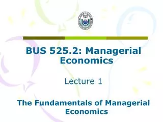
MANAGERIAL ECONOMICS Lecture 4 . Evaluating Country Economic Performance I: Stabilization Dr. Edilberto Segura Partner & Chief Economist, SigmaBleyzer President of the Board, The Bleyzer Foundation May 2011. Outline. I. Country Economic Analysis & Management

E N D
MANAGERIAL ECONOMICS Lecture 4. Evaluating Country Economic Performance I: Stabilization Dr. Edilberto Segura Partner & Chief Economist, SigmaBleyzer President of the Board, The Bleyzer Foundation May 2011.
Outline I. Country Economic Analysis & Management • Macroeconomic Stabilization • Relation between Internal and External Stability • Fiscal Policies, Current Account Deficits & Expenditures. • Expenditures (Absorption) and Foreign Debt • Introducing Money Demand and Supply l. The Monetary Balance-Sheet, Money Demand and Supply • Introducing the Financial Sector: Domestic Credit and Monetary Programming of the IMF-World Bank • Original Polak Model on Monetary Programming • Extended Monetary Programming of the IMF • The Original World Bank’s RMSM • The Merged IMF-World Bank Model: RMSM-X Model D. Size of a “Sustainable” Fiscal Deficit E. Monetary Policy and Inflation Targeting (IT) F. Rules of Thumb for Economic Sustainability
I. Country Economic Analysis • The performance of the capital markets (stocks and bonds) of an EM is affected by the soundness/strength of its economy. • Therefore, a successful investor in EMs must be able to analyze systematically the economic conditions of these countries. • A sound economy is one that has both macroeconomic stability and sustainable economic growth. • Macroeconomic Stability is defined by stable prices with low inflation (internal stability), and a stable foreign exchange rate (external stability). • Sustainable Economic Growth is defined by a high rate of GDP growth that can be maintained over a long time. • Solid macroeconomic stability and sustainable GDP growth are the two key factors affecting the performance of the stock exchange and bonds in an EM.
Assessing Country Economic Performance To assess country performance, two sets of issues need to be reviewed: (1) Actual Results in key economic areas: a. Actual Internal and External Stability Domestic Inflation Rate Stability of Foreign Exchange Rate & Balance of Payments Level of Foreign Debt in relation to GDP, Exports & Reserves b. Actual Economic Growth GDP Growth Rates and structure of sources of growth Saving Rates Investment Rates (2) The adequacy of the Policy and Institutional Framework to sustain future economic results: a. Policies to sustain internal and external economic stability; and b. Policies to sustain economic growth, which depends on policies regarding (i) economic liberalization, and (ii) public governance and institutional development. 4
Economic Stabilization Programs have been sponsored by the IMF and have been practiced since the early 1950’s to deal with balance-of-payment disequilibrium. However, in the early 1980’s, following the Debt Crises of 1982, there was wide recognition that stabilization programs alone were failing to bring back sustainable economic stability. This was because of its failure to remove deep-rooted structural economic and social distortions. That is, the balancing of fiscal budgets and B/P accounts alone were not sufficient to bring long-term stability and recovery. In order to remove these economic and social distortions, many Emerging Markets implemented Government programs to remove structural distortions in order to encourage investments and accelerate growth.
Structural Adjustment Programswere designed to achieve sustainable economic growth. They added two new elements to macroeconomic stabilization programs: 1. Economic Liberalization: These are policies to provide freedom to do business in a competitive environment (Stage 1 reforms) – In a market economy, the “motivator” is the freedom to make profits, whereas the “control system” is strong competition that discourages power abuse. 2. Institutional DevelopmentandPublic Governance: Reform of the State and Legal Systems to ensure policy implementation and to make policy changes sustainable over time (Stage 2 reforms).
Determinants of an Improved Business Environment (I) Macroeconomic Stabilization Policies: Fiscal Policies under which the Government's fiscal budget has a deficit that can be financed by borrowings on a sustainable basis (normally no more than 3% of GDP). Monetary Policies, under which the creation of money (money supply) will not exceed the demand for money (which is affected by income, prices and interest rates). (II) Structural Adjustment (A) Liberalization of the Economic Environment Liberalization of the Formation and Operation of Enterprises Liberalization of the Closure of Failing Enterprises Liberalization of Product Markets: Pricing and Trade Liberalization of Factor Markets: Capital/Financial, Labor and Land Markets (B) Sound Institutions and Public Governance Sound & efficient Government services without corruption Stable and predictable legal environment Low political risks.
Macroeconomic instability increases the risk of doing business: with unstable prices (high inflation) and unstable exchange rates, it is not possible to do financial plans and project profits. Investors will require significantly higher rates of returns to compensate for the risks of instability in prices and foreign exchange. As a result of this high risk premium, few projects would qualify for investments, reducing the overall level of investments and growth. Macroeconomic stabilization programs are based on the IMF's Monetary Approach to the Balance of Payments, which has three elements: A. The first element focuses on the government’s fiscal budget policies and the relationship between internal stability and external stability: there is a close accounting relation between the size of fiscal budget deficits, overspending by the private sector, and current account deficits.
B. The second element introduces the monetary sector. If money supply (which is controlled by the Central Bank) exceeds money demand (the amount of money that people want to hold), then people will attempt to get rid of this excess money by spending it in local goods (contributing to inflation) or importing foreign goods (leading to balance-of-payment deficits). C. The third element introduces the financial/banking sector: The excess growth of Net Domestic Credit over growth in money demand will equal the deficit in the balance of payments. • The aim of the IMF’s Monetary Programming is to determine the fiscal and monetary policies (particularly the size of the fiscal budget deficit, the growth in money supply and the level of domestic credit by the banking sector) that are “consistent” with the country’s objectives for (i) GDP growth, (ii) level of inflation, and (iii) level of international reserves.
Fiscal Budget Policy and the Relation Between Internal & External Stability Definitions: Y = Gross Domestic Product (Yncome) Yd = Gross Disposable Income (C + S) C = Consumption, private I = Investment, private G = Government Expenditures X = EXports J = Imports S = Savings, private, corporate and households T = Taxes TRf = Net TRansfers Received from Abroad (foreign) Yf = Net Factor Income from Abroad (Yncomeforeign) R = International Reserves K = Foreign Kapital A = Absorption (Expenditures) CAB = Current Account Balance
A. Fiscal Budget Policy and Internal-External Stability A economy’s Money Flow without the Government and External Sectors: Y = C + I – Sc = C + Sh → I = Sc + Sh → I = S
An economy’s money flow, with government but without the external sector. (10 - 10) = (6 – 6) G↑ by 2, then I↓ or S↑ (8 – 10) = (6 – 8) Y = C + I + G = C + S + T → (I – S) = ( T – G)
An economy’s money flow, with government and external sector. Francois Quesnay, Tableu Economique, 1758; Simon Kuznets, National Income, 1929-1932; 1934 (ed Kharkiv)
(1) On the expenditure side: AD ⇒Y = C + I + G + X - J (2) On the Income (supply) side: AS ⇒Y = C + S + T - Yf - TRf Since Aggregate Demand must equal Income, then (1)=(2); or C + I + G + X - J = C + S + T - Yf - TRf Then: X - J + Yf + TRf = (S - I) + (T - G) --------------------- ----------- --------------- Current Account Private Sector Fiscal Budget Balance (CAB) = Balance (PSB) + Balance (FBB) If PSB=0, Current Account Balance = Fiscal Budget Balance A Fiscal Deficit will yield an equally-sized CA Deficit If FBB=0, Current Account Balance = Private Sector Balance A Private Sector Deficit will yield an equal CA Deficit Note: All Savings (private sector, Gvt and foreign savings) must equal Investments for equilibrium in the goods market (I = Σ S)
1. Current Account Deficits & Excessive Expenditures. (1) Y = C + I + G + X - J Y = C + S + T - Yf - TRf = Yd + T - Yf – TRf where Yd = C + S Yd + T - Yf - TRf = C + I + G + X - J Yd - [(C + I) + (G - T)] = X - J + Yf + TRf = CAB (C + I) = Expenditures of Private Sector = Private Absorption (G - T) = Excessive Govt. Expenditures = Govt. Absorption Current Account Balance =Yd - [Priv. Abs + Govt Abs] Current Account Balance = Yd - Absorption The excess of absorption (expenditures) over disposable income will be reflected as a deficit in the current account of the B/P. To correct a B/P deficit, you need to reduce Exp. or increase Yd. A devaluation would improve the B/P if it leads to an increase in income (Yd) that is greater that an increase in expenditures (Abs), including those expenditures generated by the higher income.
2. Expenditures (Absorption) and Foreign Debt If FDIs are constant, the Current Account Deficit can be financed by: (i) a reduction in International Reserves (R), or (ii) an increase in Foreign Debt (K), assuming constant FDIs. CAB = X – J + Yf + TRf = - R + K since: CAB = Yd - Absorption therefore: Yd - Absorption = - R + K If expenditures (Absorption) are too high compared to Disposable Income, then: International Reserves would be falling or Foreign Debt would be increasing. To maintain International Reserves and avoid excessive Foreign Debt, expenditures (Absorption) should be reduced, normally by cutting Government expenditures, increasing tax revenues (reducing the fiscal budget deficit) or reducing private expenditures. All these identities are useful relationships to identify fiscal budget policies. But they provides limited guidance to monetary policy decisions. For this purpose, we need to add a number of accounting and behavioral relationships relating to the Financial/Monetary Block.
B. Introducing Money Demand and Supply In order to use the previous macroeconomic identities to define more specific fiscal and monetary Stabilization Policies, we need to introduce some key monetary and behavioral relationships concerning the Monetary Sector, including Money Demand and Money Supply. Abbreviations: Md = Money Demand: the amount of money that people want to hold (Liquidity preference). Ms = Money Supply: the amount of money issued by the monetary and banking sectors P = Prices E = Exchange Rate i = Interest rates NDCp = Net Domestic Credit to Private Sector NDCg = Net Domestic Credit to Government OIN = Other Investments, Net
Balance Sheet of the Monetary Sector A key monetary relationship is the balance-sheet of the Monetary Sector (Central Bank and Commercial banks): its Financial Assets (International Reserves, Net Domestic Credit and Net Other Investments) will equal its Financial Liabilities (Money Supply) plus Equity: Ms + Equity = R + NDCg + NDCp + NOI If Equity and ONI are fixed, then: M s = NDC + R
, The Demand for Money and the Supply of Money A key proposition is that in an economy, people have a demand function for real money - Md (currency in circulation and bank deposits), or have a "liquidity preference", which depends on real economic variables, such as the level of real income, real interest rates, rates of inflation, etc. This demand for money is determined, not by the monetary policy of the authorities, but by the public. On the supply side, there is an amount of money which is partly determined by the monetary authorities (Ms), through their discount rates, open market operations (trading of government securities) & reserve requirements. It is a key proposition that while money supply is influenced by monetary authorities, money demand is independent and determined by the people. This leads to a second proposition: when money supply exceeds money demand, the monetary balances of people exceeds their liquidity preference. Then, people will try to bring them down by spending the excess money in the purchase of local goods (which raises their prices) or in imported goods (which will put pressures on the balance of payments). Therefore, the Central Bank can reduce inflation and improve the balance of payments just by putting the monetary brakes to reduce money supply.
Formulation of the Demand for Money People will demand money (Md) to facilitate their purchasing of goods and services, which in turn will depend on their real income (Y). Therefore, money "demanded" for transactional purposes will be: Md= f (Y) But this is not the whole story, since total money demand would also depend on how much money people will be willing to hold for asset/speculative purposes. This will be a function of the cost & risks of holding money – versus other financial assets -- which depends on the level of nominal interest rates (i ), inflation (P), and the exchange rate (E). Furthermore, according to Fisher, nominal interest rates is: r + Pe The demand for money (Md) will depend on the level of real income (Y), the level of real interest rates (r), the current and expected price levels (P, Pe ), and the exchange rate (E): Md = f ( Y, r, P, Pe, E ) and in equilibrium = Ms This relationship also implies that inflation (P) depends not only of today’s Msbut also on ‘expectations” of future inflation (Cagan).
Excess Money Supply and Inflation • The Quantity Theory of Money provides and early analysis of how "excessive" money supply can lead to price increases or inflation. • It was first described by Copernicus (1526), the Salamanca School (1550), and Jean Bodin (1560) -- the last two to explain high inflation in Spain in the 1500’s due to excessive silver from Mexico & Peru. • John Locke (1692), David Hume (1748) and John Stuart Mills (1848) described precisely the relation between money supply and the value of money transactions. • It was formulated as an equation by Irving Fisher (1911) and reformulated in its modern version by Milton Friedman (1956). • The main points can de described as follows: • In the economy there are 100 monetary units (M), which are spent exclusively in the purchase of goods. • In this economy the quantity of goods sold (Q) is 100 goods per year. • Then, the price of each good sold (P) will be 1 monetary unit (P). • Later on, the government prints money and the amount of money goes to 200 monetary units, but there are still 100 goods sold.
Then the price of each good will be 2 monetary units: a 100% inflation rate. Therefore: M = P x Q • Since this assumed a transaction velocity of money of 1, generalizing to a velocity different to one (Vt) - which implies a changing Money Demand, we get the formulation of the Quantitative Theory of Money: M x Vt = P x Q • Since the amount sold (Q) is proportional to the amount produced (Y): M x V = P x Y where V is now the income velocity of money. • Considering changes: (1+ M) x (1+ V) = (1+ P) x ( 1+ Y) • or: P = f (M, V, - Y) if Money demand is constant (V=0) and Y=0; then P = f (M) • If the amount of money in the economy grows by 20%, real GDP grows by 3%, and money demand is constant (velocity is constant), then inflation will be 16.5%, (ie, 1.20/1.03).
In the UK, a 1% increase in interest rates will produce a 0.2%-0.3% decline in GDP in one year, and a 0.2%-0.4% decline in inflation after two years.
Other Useful Relationships 1. The amount of Imports will depend on the level of Income. J = Y where is the import elasticity 2. Income will depend on the level of Investments, which will also depend on the level of domestic credit to the private sector. 3. Given a "desired" level of income, the NDC needed by the private sector is also defined: NDC p = Y
C. Introducing the Financial Sector and Domestic Credit The Original Polak Model for Monetary Programming
C1. Introducing the Financial Sector and Domestic Credit:The Original Polak Model on Monetary Programming The original IMF Monetary Programming (developed in 1957) was designed for BOP crises prevention & resolution, not growth. It therefore focused on the Financial and Balance of Payments blocks, ignoring the Government and Private Sector blocks. The objective was the level of Reserves, given an income growth. It assumed fixed exchange rate regimes - the regimes in the time. Reserves are key to credibility of fixed ERRs (Krugman [1979]) Control over net domestic credit expansion is the key to stabilize the level of reserves and therefore the Balance of Payments. Described by Four Equations (1) to (4): M s =M d (1) M s = NDC + R (2) M d = f (Y) = v -1Y v > 0(3) R = X - J + K =X - Y + K 0 < < 1(4) Also: If M s>M d then: (1) P↑, J↑, X↓ and R↓ and also (2) people will reduce the excess money in tradables: J↑ and R↓
Focusof the Polak Model: To determine the effects of changes of net domestic credit on reserves. Using (1), (2), and (3), one gets: R = M s - NDC = M d - NDC R = v -1Y - NDC Reserves will decline (B/P deficit) when increases in net domestic credit (NDC) exceeds increases in nominal money demanded (M d), which in turn depends on the rate of income growth (Y) . Reserves stable if growth of domestic credit ⇒ nominal output growth If Y grows, M dwill grow and NDC can grow somewhat with R stable. But if NDC grows over and above grow in Md, then R will fall. Management of net domestic credit is crucial in obtaining BOP objective: NDC = v -1Ytarget - Rtarget Given a target level of income growth (Y), and a target level of reserves (R) one can estimate the required change in NDC This allows policy makers to estimate a credit ceiling, i.e. Net Domestic Credit growth is a performance criterion in IMF programs Transmission channels: Assuming that Y↑ J↑ CAB deteriorates R↓ then, if: NDC↓ Ms↓ Md>Ms i↑ I↓ AD↓ J↓ CAB improves R↑; also as: i↑ K↑ R↑ ⇒A reduction of NDC lead to improved B/P
C2. Extended Monetary Programming of the IMF In the 1970’s, the model introduced the effects of changes in Prices & Exchange Rates (given the abandonment of fixed exchange rates in 1973.) It also introduced the Government’s fiscal block: Govt Revenues (T) – Govt Expenditures (G) = Fiscal Balance = NDCg + Kg
Maximum Domestic Credit to the Government Taking the Balance Sheet of the Banking Sector: Ms + NW = R + NDCp + NDCg + OIN Ms = R + NDCp + NDCg,-since NW & OIN are fixed. Ms is defined from its identity to money demand, given interest rates and targets on inflation and income. R is a target and is defined by the outcome of the Balance of Payments. NDCpis defined by the requirements for working Cap/income growth of the private sector. Therefore, NDCg will be the residual amount. This residual amount, Net Domestic Credit to Govt., is all the lending from domestic sources that can be given to the Government if the country were to have equilibrium in the money markets (inflation at target level). The size of a “consistent” fiscal deficit will depend on the amount of financing available: the amount of NDCg plus any additional foreign loans that the Government may obtain. T – G = NDCg + Kg This model is still widely used by the IMF. BUT: it ignores equilibrium in the non-financial private sector (good markets -- I and S)
C3. The Original World Bank’s RMSM (Revised Minimum Standard Model) Developed in the early 1970s (Chenery & Strout) with the objective of making explicit the link between medium-term growth and equilibrium in the goods markets Economic Growth is the key target, along with the level of Reserves (to avoid BOP crisis). It is forward looking focused on the savings-investment gap. But it ignored the monetary and financial sectors. Assumptions & Growth Theory behind the RMSM: Linear positive relation between investment and output growth rates (Harrod–Domar, endogenous growth models). Emphasis on capital accumulation and its effects on Income through an Incremental Capital-Output ratio (which can vary in the future). Additional foreign flows go to investment (Chenery and Strout [1966] model)
Five relationships define the RMSM model: National income identity: y = y-1 + y = C p + I + G + (X - J) (1) Private consumption: C p = (1 - s)(y - T) 0 < s < 1: marginal propensity to save (2) T = taxes Investment: I = y / : inverse of the incremental capital-output ratio (3) Imports: J = y 0 < < 1 (4) Balance-of-payments identity: X - J = R - K (5)
Target equations (derived by substitutions): (s + )y-1+ (1 - s)T - (X + G) ________________________ (yy) -1 - (s + ) R= X - (y-1 + y) + K (bb) The structure of RMSM: Target variables: y, R (Macroeconomic Objectives) Exogenous variables: X Policy instruments: G, T, K Predetermined: y-1 Parameters: ICOR ( -1), marginal propensity to save (s), and import elasticity ( ) Endogenous variables: I, C p, J y =
These two Equations can be solved (i.e. a numerical y and R can be obtained) in a Simultaneous Mode or in a Recursive Mode: Simultaneous mode: The first equation will give y (growth rate) for a given y -1, X, and the policies T and G. Then substituting this y into the second equation, will give R for a given K (or viceversa). Recursive or Programming mode: Set targets for income growth and R and given y -1, X, T and G, through recursive (iterative) solution, calculate K = financing needs. Alternatively, can use same approach to get G [if Y = f(G, J), we can reverse it for G = f-1(Ytarget, J)]. Criticisms of RMSM: Difficult to identify the binding constraint a priori. Assumes that import constraint as essential for income growth and investments; however, the foreign trade gap can also be closed by exports increases, thereby providing foreign exchange necessary for investment. Neglects relative prices and induced substitution effects among production factors (and their possible impact on exports). Incomplete: a growth-oriented model with emphasis on a small number of real variables but no government side and no monetary side, hence no use of huge literature on this relation.
Adds the World Bank’s RMSM to the IMF’s Monetary Programming model. It covers the four major blocks: Monetary, Govt., B/P, and private sector. As in the IMF Extended model, relative prices and the exchange rate affect imports and domestic absorption. Basic Model Equations: (1) Money supply and domestic credit M s= NDC p + NDC g+ R, with NDC p = Y (Credit proportion for working capital) and R = E R* (2) Money demand M d = v-1Y (3) Flow equilibrium of the money market M s= M d (4) Government budget financing constraint G - T = NDC g + K g C4. The Merged IMF-World Bank Model:The RMSM-X Model
(5) Balance of payments R = X - J + K with: K = E K*,and: X is exogenous. Nominal imports: J = J-1+ (QJ-1 - E-1)E + E-1(y + PD) With (Q) as import volume, () price elasticity of imports and () income elasticity of imports (see Note 1). (6) Changes in investments, output and prices I/P = y/ where I is Nominal Investment & -1 is the ICOR Y = Pywhere Y & y are Nominal & Real Income Y = Py - P-1 y-1 = Py - P-1 (y - y ) ≈Py-1+ P-1y and: P = PD + (1 - )(E + P*) (weighting P and P*) Where: is the relative weight of domestic goods in the price index (1- ) is the proportion of imports (devaluation pass-through effect). P is domestic inflation and depends on the weighted domestic prices (PD) and foreign prices (P*) P* is foreign inflation which is thereafter assumed to be zero.
(7) Private sector budget constraint: Starting from the national income identities: AD = Y = C p + I + G + (X - J) AS = Y = C p + S + T - Yf - TRf Since AD = AS: (I-S) + (G-T) = - (X - J + Yf + TRf) = CAB Since CAB = K - R: (I-S) + (G-T) = K - R Since: K = K p +K g and: R = Ms - NDC Ms = Md NDC = NDCg + NDC p Then: (I-S) + (G-T) = K p +K g - Md + NDCg + NDC p Since (G-T) = K g + NDCg from equation (4) Then: I – S = NDC p + K p - M d Which defines the private sector budget constraint: The excess of private investments over private savings must be financed from net domestic credit to the private sector (NDC p), foreign capital for the private sector (K p), and/or by a reduction in the demand for money.
Model Consistency Another way of looking at the above is to combine the Government and Private Sector budget constraints in equations (4) & (7) to give the overall budget constraint for the economy (or savings-investment balance). This balance relates total savings (public and private) and investments to domestic & foreign financing (NDC g, NDC p, Md and Kp). In fact, with some transformations, we obtain the sum of equations (4) and (7) as the following: (I-S) + (G-T) = NDC + K - Md Since NDC= Ms - R and Md = Ms, then: (I-S) + (G-T) = K - R = CAB As we saw earlier, this last equation implies that the Monetary and National Income identities do hold (that is, Md = Ms and that AS = AD; I = Σ S: AD = AS = Y = C p + G + I + (X - J) = C p + S + T - Yf - TRf
Footnote 1: Imports under the RMSM-X J = E QJ(with P*J= 1) J: imports in nominal terns; QJ: import volume; E : nominal exchange rate Changes in import volume depend on the change in real income (y) and the relative price of domestic and foreign goods: QJ= y + [PD- (E + P*)] > 0: import elasticity to relative price changes. Nominal value of imports: J QJ-1E+ E-1QJ so that: J = J-1 + (QJ-1 - E-1)E + E-1[y + (PD - P*)] With QJ-1 relatively small, a devaluation in the nominal exchange rate (E > 0) will lower the nominal value of imports, improve the trade balance and thus increase official reserves. The last term of the equation can be dropped if we assumed that foreign inflation is small. 43
Structure of the Merged Model: Target Variables: y, PD , R Endogenous Variables: Y, NDCp, M, P, J, T Exogenous Variables: X, K = Kp + Kg Policy Instruments: NDCg, E, and G Predetermined: y-1, P-1 Parameters: money velocity (), devaluation pass-through (), coefficient of credit proportion for working capital (), price elasticity of imports(), income elasticity of imports (), incremental capital-output ratio( -1), marginal propensity to save (s). Solution of the Merged Model: Objective is to relate targets, exogenous variables, and policy instruments to find the equilibrium values for y, PD and R (in which Md=Ms and I=ΣS). Starting with the private sector budget constraint (7) in the Basic Model, S - I = Md - NDC p - K p But since S= Y- C p – T: Then: (Y – C p - T) - I = Md - NDC p - K p Since C p = (1 - s)(Y - T) where s is the marginal propensity to save. Then: I = s(Y-1 + Y - T) + NDC p + Kp - Md but since Md = v-1Y Then: I = s(Y-1 + Y - T) + NDC p + Kp - v-1Y Re-arranging and using credit to private sector, NDC p = Y, and assuming = s + - v-1 is positive (or v(s + )>1), we obtain the target equations of the Merged Model by substitutions in the Basic Model equations.
Target Equations of the RMSM-X Model - + (-1 - )y - (1 - )-1E (1) PD = y-1 (yy) where: = sY-1 + (1 - s)T - G +K + NDCg (2) R + (-s)(y-1PD + y) = -(-s) y-1 (1 - ) E - NDCg (mm) (3) R = X - J-1 - (QJ-1 - E-1)E - E-1(y + PD) + K (bb) • Equation (1) relates PDandy based on equilibrium in the goods market (equation (7) of the Basic Model with I=ΣS) (the yy curve in the chart) • Equation (2) relates R and y based on equilibrium in money markets (equation (3) of the Basic Model with Md=Ms) (the mm curve in the chart) • Equation (3) also relates R and y but based on equilibrium in the balance of payments (equation (5) of the Basic Model) (the bb curve in the chart) • These equations can be solved in a simultaneous or in a recursive basis. • From these equations, one can see that a change in the policy instruments • (G, NDCg and E) changes the equilibrium solution for y, PD and R
The above chart shows the simultaneous solution for the RMSM-X at equilibrium points E-A (giving y*, PD* and R*) If the decision makers want to change the solution from points E-A to points E1- A1, this can be achieve through a combination of changes in the exogenous policy variables G, NDCg and E. But to achieve final equilibrium, all these policy variables need to be adjusted.
Principles of Recursive (Programming) Solution Income growth (y), domestic price level (PD), and reserves (R) are targets. Policy Instruments are the government budget (G), the exchange rate (E), and net credit to the government (NDCg) To increase output, lower inflation, and increase reserves reduce government spending, G, devalue exchange rate, E or lower NDCg. Other examples of analysis: Increasing NDC (domestic credit) to achieve higher growth will just result in higher inflation: δy/δNDC > 0 ; but δPD /δNDC > 0 To get higher reserves, reduce income growth and/or domestic credit, and devalue: δR/δy < 0; δR/δNDC < 0; To achieve higher reserves, lower Government spending: δR/δG < 0
Consists of four economic sectors: the public sector, the private sector, the consolidated banking system, and the external sector. Each sector is subject to its own budget constraints. National accounts, derived via aggregation of the sectoral budget constraints, serve to close the RMSM-X model. Two types of financial assets (money and foreign assets) in a standard model. For middle-income countries, some models include bonds. The money demand function frequently follows Polak Model in assuming constant income velocity of money. Some models disaggregate the banking system structure: instead of Ms = NDC + R, Ms is rather obtained as the product of the monetary base and a constant money multiplier. Imports consist of several categories with the demand for imports a function of the real exchange rate and either real GDP or gross domestic investment (for imports of equipment). Consumption is generally assumed to depend only on disposable income -- thereby excluding consumption-smoothing effects. Investments is based on a simple ICOR formula General characteristics of the RMSM-X model:
Steps to Carry out Monetary Programming (1) Evaluate Economic Problems: nature/source of imbalances. (2) Identify exogenous factors: world economy/trading partners. (3) Set preliminary targets for the objectives of the country in terms of (a) GDP growth, (b) inflation and (c) level of International Reserves and set a preliminary policy package for other variables. (4) Formulate a monetary program: money demand, banking sector. (5) Prepare a balance of payment forecast: exports, imports, capital. Prepare a fiscal budget forecast: Govt revenues, expenditures. Prepare the private sector block balance, calculating investment requirements, given estimates of ICOR and income growth rate. (8) Ensure consistency of forecasts with accounting and behavioral identities, through a recursive (iterative) process until you reach a fully consistent program, including external financing from IFIs. (9) Review the conditionality attached to required external financing (IMF, IBRD), and decide how to monitor the program: prior actions, performance criteria, structural benchmarks, reviews.
Policy Options if the RMSM-X Model shows a Fiscal Gap If the fiscal deficit is higher that the amount of financing available, the Government has only four alternative policy options: 1. To reduce Government expenditures 2. To increase Government revenues 3. To change other conditions in the economy to yield a larger volume of financing to the Government, such as: reduce credit to the private sector, increase money demand (by increasing growth, reducing interest rates and allowing higher inflation). 4. To print money, which will lead to inflation. The “quality” of the measures to be taken to achieve a reduction in the deficit and achieve equilibrium is fundamental for the economic, social and political sustainability of the program.