Download
1 / 15
150 likes | 286 Views
This paper discusses a novel approach to real-time traffic density estimation using GPS data from vehicles. By collecting position data, a central mobility management system computes density around specific locations, weighing contributions based on vehicle proximity. Challenges such as the unsustainable communication load between numerous devices and the adaptability of "Safe Zones" for vehicles are also addressed. The framework incorporates adaptive learning from historical data to enhance predictive accuracy of user mobility, significantly reducing the need for constant communication while maintaining performance.

E N D
Efficient distributed computation of human mobilityaggregates through user mobility profiles Mirco Nanni, Roberto Trasarti, Giulio Rossetti, Dino Pedreschi KDD Lab - ISTI CNR Pisa, Italy
Objective and Motivations Reference application: real-time traffic density estimation at key locations Possible approach: Exploit on board GPS devices GPS devices can transmit their position real-time to the mobility management central The mobility management central uses collected positions to compute the density around a specified set of locations Vehicles closer to the location contribute to density with higher weight
Issues Central Server GSM network GPS Devices Mobility data come from large number of devices on the territory. The communications between these devices and the central server is unsustainable.
Outline of Approach: Global function Density estimation of each reference point RPi based on some kernel K Basic case: radial function, e.g. Gaussian nV = n. vehicles Vixy = vehicle positions RPixy = RP positions • Error tolerance: each density is computed with approximation ε
Level 0: Static “Safe Zones” Compute a “default location area” around the most frequent (dense) location, from historical data Safe zone = default location ± ε/N Whenever the vehicle is inside the area, no communication occurs Level 1: Adaptive “Safe Zones” As above, but when a vehicle exits its SZ, a new one is computed, centered around the last location sent Which “intelligence” to put into the framework?
Level 2: Learn from historical data Try to exploit the high predictability of human mobility1 Level 2.1 Assumption: “Average user tends to visit (or cross) everyday the same places at the same hour of the day” Single spatio-temporal locations need not to be linked Level 2.2 Assumption: “Average user tends to repeat the same trips everyday” The “regular trip” is an higher level concept, requires a coherent sequence of spatio-temporal locations 1 - C. Song, Z. Qu, N. Blumm, A.-L. Barabási. Limits of Predictability in Human Mobility. Science Which “intelligence” to put into the framework?
Level 2.1: Most Frequent Location Model For each user: Discretize and align daily movements into time slots of M minutes each to obtain a complete schedule for each day; Assign to each time slot the corresponding most frequent position – thresholds on distance and min frequency required Which “intelligence” to put into the framework? (x,y) (x’,y’) (x”,y”) Daily schedules (x,y) (x,y) (x”,y”) Frequency based profile (x,y) (x”,y”)
Which “intelligence” to put into the framework? • Level 2.2: Mobility profiles • The central controller is provided with “Mobility profiles” individually extracted from the history of each vehicle2 Trajectories of the individual Extracted mobility profiles 2 - Roberto Trasarti, FoscaGiannotti, MircoNanni, Fabio Pinelli: Mining mobility user profiles for car pooling. KDD 2011
Outline of Approach: Flow of the application Each vehicle computes its model and sends it to the Controller The Controller sends to each vehicle an error ε' Basic solution: ε' = ε / nV in the worst-case scenario Loop: Each vehicle evaluates, for each RP, its kernel contribution K based on its actual position, and contribution K' based on predicted position. If |K-K'|>ε' sends a correction: In case of profiles: a temporal shift dt, if the vehicle is slightly late/early In case of frequent location or large dt: the actual position (x,y) or its Ks The Controller evaluates the kernel contributions based on the model (aligned through dt, if based on profiles) or last position of each vehicle
Experiments GPS real car users around 40,000 users locate in Tuscany time period of 5 weeks mixed territories Data by OCTOTELEMATICS Approaches compared: Level 1 (Adaptive Szs) Level 2.1 (Freq. Locations) Level 2.2 (Profiles) RPs used in experiments
Experiments Lev. 2.2 vs Lev. 1
Experiments Lev. 2.1 vs Lev. 1
Experiments Lev. 2 vs Lev. 1
Conclusion and Future Works SUMMARY • Several approaches to the problem of computing population density over key areas have been proposed using different levels of “intelligence” • Significant reduction in communications was achieved • The results suggest that a high level knowledge boosts to the performances ONGOING WORKS • Can the proposed framework be made privacy-preserving? • Are there parts of the map more difficult to "learn"? • E.g. Highways are expected to be difficult, due to high presence of occasional trips and passers-by • If taken collectively, individual non-systematic behaviors might form typical paths, e.g. vehicles on the highways: how to integrate them in the framework?
Thanks! Questions? kdd.isti.cnr.it/ www.lift-eu.org/ giulio.rossetti@isti.cnr.it