Download
1 / 40
420 likes | 578 Views
Neural Networks. CIS 488/588 Bruce R. Maxim UM-Dearborn. Neural Networks. Can be thought of as arithmetic constraint networks Tend to be designed in layers Input layer Hidden layers (1 or more) Output layer. Neural Network Types. Feed-forward

E N D
Neural Networks CIS 488/588 Bruce R. Maxim UM-Dearborn
Neural Networks • Can be thought of as arithmetic constraint networks • Tend to be designed in layers • Input layer • Hidden layers (1 or more) • Output layer
Neural Network Types • Feed-forward • Input signals travel though input layer, hidden layers, and output layer • Require training • Thought to simulate learning • Feedback • Network pays attention to it own results and uses the results to adjust errors • Tend to be constructed rather than trained • Thought to simulate “instinctual” behavior
Feedforward NN • Input neurons calculate output values and pass them forward to the next layer • Each hidden neuron adds up the signals from every input neuron using its own weightings • New signal passed own to all neurons in the next layer • Output layer neurons compute final values based on summing signals from the last hidden layer using their own weights and formats the signals for display
Neural Nets • Activation function • Used to combine the neurons inputs and generate an output signal • Threshold function • Checks each input symbol to see if it is above or below the threshold value (signals below threshold values are ignored)
Connection Weights • Excitatory • Large positive value • Indicates strong connection • Inhibitory • Small negative value • Indicates weak connection
Neural Nets • Each neuron must store connections strengths for each neuron in the previous layer • If current layer has N neurons and previous layer has M neurons connection strength storage requires N*M words • All neural network knowledge is contained in its connection weights which are modified as the result of training
Learning • Supervised Learning NN receives some type of signal or pattern is present to tell neural net whether output is correct or not • Unsupervised Learning No such signal is present
Training - 1 • Involves modifying the connection weights in an orderly manner • Training sets (fact sets) should be developed while neural net is being designed • Facts consist of input/output pairs for supervised learning • For unsupervised learning output pattern is not present
Training - 2 • Basically NN processes facts one at a time and modifies its connection weights • Typically NN need to trained more than once using the same set of facts • Process continues until connection weights stop changing • For supervised learning the differences between the NN output and the fact output causes NN to modify its weights to try to reduce its errors
Using Neural Nets • Once the neural network is trained it can generalize its experiences to new cases • A small network (say 10 or fewer neurons) will not be very good at generalization
Learning Algorithms • Linear algorithms • Have one to one connections between their neurons • Non-linear algorithms • Have many to many connections among their neurons
Peceptron Algorithm - 1 • Given: classification problem with N inputs and 2 outputs • Task: compute set of weights for inputs matching first output class Algorithm: 1.Create perceptron with N+1 inputs and N+1 weights 2.Initialize weights with random values
Peceptron Algorithm - 2 3.Iterate through training set and save all “misclassified” facts 4.If all facts correctly classified then output weights and stop 5.If some examples not classified correctly then compute vector sum of bad input facts 6.Adjust weights using vector sum 7.Go to step 3
Perceptrons - 1 • Tend to be built in single layer though multiple layers are possible • Neurons take their input from any other neuron and can process their own outputs • Computations are repeated over and over until weights reach equilibrium state • They are good at reconstructing facts from incomplete or error filled input • They are memory intensive given their limited capacities
Perceptrons - 2 • Multiple outputs can be handles using the same principle • All outputs are independent from one another • The weights 1 through n are connected to the inputs • Weight w0=b is not connected to an input and is known as the bias or constant offset • For implementation a dummy input set to 1 is connected to the bias weight
Perceptrons - 3 • Traditional neural networks use binary values for inputs and outputs, with floating point numbers for the weights • Game developers tend to use 64bit floating point numbers for all three • The FEAR use 32bit float point numbers to speed up computation and reduce storage
Simulation • Net Sum = w0 + wixi x0 = 1 • Activation Function (x) = 1 if x > 0 or 0 otherwise • Keeping all numbers as floating point values allow for smoother movement control
Perceptron Algorithm net_sum = 0; for i = 1 to n net_sum += input[i] * weight[i]; output = activation(net_sum); • Output can be used to evaluate the suitability of a behavior or to determine when a situation may be dangerous • Weight optimization is needed to approximate a function correctly
Optimization • The task might be to determine where the NPC should shoot to inflict maximal damage • You could conduct controlled experiments with varying parameters and measure the damage • How ever this would only be for a single situation and you could miss the optimal point if the input value falls within the increment used for the values
Steepest Descent • An iterative technique based on slope of function • Seeks to find x value such that f(x) is a global minimum • Stopping condition |xi+1 – xi| <= • xi+1 = xi + xi = xi - f(xi) • f(xi) is the gradient (slope) of the function and is the learning rate used to scale each iteration
Learning Rate • Large values of can cause fast convergence for simple functions • Large values can cause oscillations for certain functions • Small values of will force more iterations to obtain convergence • Values need to be chosen on a case by case basis (there is no one good value for )
Local Minima • Similar to the foothill problem in hill climbing • It is hard to distinguish local minima from a global minimum, just looking at the nearby values • Triggering the halting condition early is quite likely and is worse when gradient function is oscillating • AI algorithms really need clear solutions to problems to work well
Momentum • One way to prevent premature convergence into account is to consider momentum (like a ball rolling up and down the foothills) • This is done by giving the algorithm a short-term history to examine when choosing the next step • This is done by scaling the previous by and using it with gradient learning rate xi = xi-1 - f(xi)
Simulating Annealing - 1 • This approach is not gradient-based, though slope information can be added • Modeled after cooling metal as it settles into a configuration that minimizes its energy • Method is based on choas theory, estimate for the next generation is based on a guess • A generation mechanism stochastically picks a new estimate in the neighborhood of the current estimate
Simulating Annealing - 2 • p is the probability of choosing the new estimate over the current on is based on the temperature T, k is a constant p = exp(- f / kT) • In theory the optimization will settle into a global minimum as the temperature decreases • If p=0 simulated annealing is really just greedy hill climbing
Optimizing Perceptron Weights • To get the outputs right we can • Use training • Encourage imitation • Automated learning (from another AI) • Previous results (boot strapping) • Each output estimate is based on a set of weights • If comparing the actual output to desired output indicates an error the weights are corrected using the delta rule
Delta Rule – 1 • Each observation contributes a variable amount to the output • The scale of the contribution depends on the input • Output errors can be blamed on the weights • A least mean square (LSM) error function can be defined (ideally it should be zero) E = ½ (t – y)2
Delta Rule – 2 • The gradient of error E relative to wi can be computed E/wi = - xi (t – y) • We could adjust the weights using a method like steepest descent wi = - E/wi = xi (t – y)
Training Procedure • Uses weight optimization to produce the desired neural network • The aim of training is to satisfy some objective function that evaluates the quality of the networks • Three data sets may be used (one for training, one for validation after training, and one for testing)
Training Algorithm initialize weights randomly; while (object function not satisfied) for each sample { stimulate perceptron; if (result is invalid) for i = 1 to n { delta = desired – output; weights[i]+= learning_rate * delta * inputs[i]; } }
Delta Rule Batch Training Algorithm - 1 while (termination condition not verified) { reset steps array to 0 for each training sample { compute perceptron output for each weight i { delta = desired – output; steps[i] += delta * inputs[i]; } }
Delta Rule Batch Training Algorithm - 2 for each weight I weights[i]+= learning_rate * steps[i]; } • Mathematically this corresponds to gradient descent on the quadratic error surface • Error is minimized globally for entire data set, and best result will always be reached if algorithm terminates
Summary • Perceptrons provide easy solutions to linear problems • Main decision is between the two algorithms (perceptron training and batched delta rule) • Both algorithms find solutions is they exist, given a small enough learning rate • Delta rule is preferred when all data sets are available for training (sometimes wise to discard successful cases as they are learned)
Major Pain • Uses a simple perceptron to learn to fire • Perceptron needs to learn that it is OK to fire when an enemy is present and the perceptron’s weapon is ready to fire • This is accomplished when the perceptron learns to compute the AND operation for two inputs