Download
1 / 28
280 likes | 472 Views
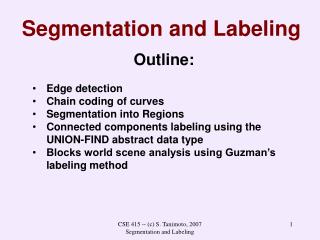
Segmentation and Labeling. Outline: Edge detection Chain coding of curves Segmentation into Regions Connected components labeling using the UNION-FIND abstract data type Blocks world scene analysis using Guzman’s labeling method. Edge Detection.

E N D
Segmentation and Labeling • Outline: • Edge detection • Chain coding of curves • Segmentation into Regions • Connected components labeling using the UNION-FIND abstract data type • Blocks world scene analysis using Guzman’s labeling method CSE 415 -- (c) S. Tanimoto, 2007 Segmentation and Labeling
Edge Detection Rationale: In order to find out where the objects are and what their properties are, locate their boundaries by finding “edges”. An edge is a transition from a region of one predominant color or texture to another predominant color or texture. Approaches: 1. local difference operators. E.g., Sobel, Roberts. * 2. model fitting. E.g., Hueckel, Canny. 3. vector space transformation. E.g., Frei & Chen. 3. contour finding via search. 4. snakes. CSE 415 -- (c) S. Tanimoto, 2007 Segmentation and Labeling
Edge Detection (cont.)Local Difference Operators (Oriented) Horizontal differences: Eh[i, j] = F[i, j] – F[i, j-1] Vertical differences: Ev[i, j] = F[i, j] – F[i-1, j] CSE 415 -- (c) S. Tanimoto, 2007 Segmentation and Labeling
Edge Detection (cont.)Combining directions Strength[i,j] = sqrt( Eh2 + Ev2) Direction[i,j] = arctan(Ev / Eh ) (note: the latter has a bug when Eh = 0. This can be fixed using alternative cases.) CSE 415 -- (c) S. Tanimoto, 2007 Segmentation and Labeling
Edge Detection (cont.)Local Difference Operators (Omnidirectional) Roberts Cross operator: E[i, j] = sqrt( (F[i, j] – F[i+1, j+1])2 + (F[i, j+1] – F[i+1, j])2 ) Sobel operator: E[i, j] = sqrt( [(c+2f+i)-(a+2d+g)]2 + [(g+2h+i)-(a+2b+c)]2) a b c b e f c h i CSE 415 -- (c) S. Tanimoto, 2007 Segmentation and Labeling
Chain Coding of Contours A chain code is a system for representing elementary vectors by small integers. = 0 = 1 = 2 = 3 To represent a curve, first approximate it as a sequence of elementary vectors, and then write down the code number for each vector in a sequence. CSE 415 -- (c) S. Tanimoto, 2007 Segmentation and Labeling
Segmentation into Regions Technique 1: Thresholding Technique 2: Region growing Example: Connected-components labeling with the UNION-FIND abstract data type. CSE 415 -- (c) S. Tanimoto, 2007 Segmentation and Labeling
Thresholding Assumption: We have a monochrome image each of whose pixels belong either to the figure(s) or to the background. Perform a thresholding transformation: T[i,j] = 0 if F[i,j] < 1 otherwise The value is called a threshold. CSE 415 -- (c) S. Tanimoto, 2007 Segmentation and Labeling
Threshold Selection Choosing a suitable can be challenging. If is too low, many pixels may be misclassified as figure, whereas, if it is too high, many pixels may be misclassified as background. The valley method: If the histogram of the input image is bimodal, choose as the threshold, the value between the modes where the histogram is lowest. CSE 415 -- (c) S. Tanimoto, 2007 Segmentation and Labeling
Valley Method Example 2 3 5 1 1 7 6 2 5 5 6 1 1 5 1 2 X X X X X X X X X X X X X X X X 1 2 3 4 5 6 7 Modes at 1 and 5. Valley at = 4. CSE 415 -- (c) S. Tanimoto, 2007 Segmentation and Labeling
Valley Method Example Result of thresholding with = 4 0 0 1 0 0 1 1 0 1 1 1 0 0 1 0 0 CSE 415 -- (c) S. Tanimoto, 2007 Segmentation and Labeling
Segmentation into Regions: A segmentation into regions means dividing up all the pixels of an image into groups. Each group of pixels must be connected to each other rather than separated in different parts of the image. Each group must have the same brightness, color, or other local property. It should not be possible to merge two groups and have the new group be both connected and uniform in property. CSE 415 -- (c) S. Tanimoto, 2007 Segmentation and Labeling
Segmentation into Regions:Formal Definitions “Adjacency” a b c d e f g h i Pixel e is 4-adjacent to each of b, d, f, and h. a b c def g h i Pixel e is 8-adjacent to each of a, b, c, d, f, g, h, i. CSE 415 -- (c) S. Tanimoto, 2007 Segmentation and Labeling
Segmentation into Regions:Connectivity Let I = {p0, p1, …, pN-1} be an image. Let R be a nonempty subset of I. Suppose R has at least two pixels. Let ps1 and psn be two pixels in R. Pixels ps1 and psn are 4-connected in R provided there is a sequence of pixels (ps1, ps2, … psn) such that each successive pair of pixels is 4-adjacent, and all these pixels are in R. CSE 415 -- (c) S. Tanimoto, 2007 Segmentation and Labeling
Segmentation into Regions:Definition of Region A region R of I is a 4-connected nonempty subset of I, such that every pair of pixels in R is 4-connected in R. CSE 415 -- (c) S. Tanimoto, 2007 Segmentation and Labeling
Region Adjacency Let Ri and Rj be disjoint regions. If pi is a pixel in Ri and pj is a pixel in Rj, and pi is 4-adjacent to pj, then regions Ri and Rj are adjacent to one another. Then we write Ri adj Rj . CSE 415 -- (c) S. Tanimoto, 2007 Segmentation and Labeling
Segmentation Definition Let I = {p0, p1, …, pN-1} be an image. Let S = {R1, R2, …, Rk} be a set of regions of I. Let P be a uniformity predicate where P(R) is true provided that all the pixels in R have a uniform appearance. For example, P(R) could be defined to be true whenever all pixels in R have the same value. S is a segmentation of I provided that: (1) The regions cover I. That is, R1 R2 … Rk = I. (2) The regions are disjoint. i j Ri Rj = . (3) Each region is uniform. j, P(Rj). (4) Segments are maximal. If Ri adj Rj then P(Ri Rj). This means no regions can be merged and still maintain uniformity within the resulting region. CSE 415 -- (c) S. Tanimoto, 2007 Segmentation and Labeling
Computing a Segmentation with the UNION-FIND ADT Initialize a set of regions by putting each pixel in its own region. Scan the image in raster-scan order. At each pixel pi, check its neighbor pj to the west (if it has one) as follows: If the two pixels have the same pixel value, do a FIND on each one getting ci and cj. If ci cj, then perform UNION(ci, cj). Then check its neighbor pq to the north (if it has one) in the same way. Perform a second scan of the image and at each pixel p, replace the pixel value by FIND(p) CSE 415 -- (c) S. Tanimoto, 2007 Segmentation and Labeling
Vision: Scene Labeling Structure in the world allows us to interpret complex situations by propagating constraints. This is conveniently demonstrated in computer vision, using a technique known as Guzman labeling. CSE 415 -- (c) S. Tanimoto, 2007 Segmentation and Labeling
Blocks-World Vision Problem Given: A 2-D line drawing representing a collection of polyhedral blocks on a table. Determine: Which faces (bounded regions in the drawing) go together as parts of the same objects. Which edges (line segments) are internal to objects and which are “occluding” edges. CSE 415 -- (c) S. Tanimoto, 2007 Segmentation and Labeling
Example Scene Analysis Problem CSE 415 -- (c) S. Tanimoto, 2007 Segmentation and Labeling
Guzman’s Vertex Labels Ell Arrow Fork Tee Arrow: There is an angle of more than 180 deg. Fork: Each of the 3 angles is of less than 180 deg. Tee: There is one angle of exactly 180 deg., and 2 smaller ones. CSE 415 -- (c) S. Tanimoto, 2007 Segmentation and Labeling
Guzman’s Labelling Technique 1. Classify each vertex into one of the categories: ell, arrow, fork, tee, or other. 2. At each vertex, mark each incoming edge according to the role it plays at the vertex (e.g., shank of an arrow, stem of a tee). 3. Create single links between neighboring regions each time: a. they are divided by a line segment at a fork, b. they are divided by the shank of an arrow, c. they are in corresponding positions of a configuration of two opposing tees with colinear stems. 4. Create a “node” for each region. Whenever two regions are doubly linked, connect their nodes with a “same object” link. CSE 415 -- (c) S. Tanimoto, 2007 Segmentation and Labeling
Example with Vertex Labels L L A A A T T F L T A T F T L L L A A CSE 415 -- (c) S. Tanimoto, 2007 Segmentation and Labeling
Example with Region Links CSE 415 -- (c) S. Tanimoto, 2007 Segmentation and Labeling
Example with Object Links CSE 415 -- (c) S. Tanimoto, 2007 Segmentation and Labeling
Example with Internal and Occluding Edges Identified internal occluding CSE 415 -- (c) S. Tanimoto, 2007 Segmentation and Labeling
Discussion The work of Guzman was refined by D. Huffman, M. Clowes, and D. Waltz to take into account additional kinds of edges, including crack edges, oriented occluding edges, and concave and convex internal edges. A key point of this research was to show that constraints imposed by the real world could make seemingly intractable combinatorial interpretation problems actually solvable. CSE 415 -- (c) S. Tanimoto, 2007 Segmentation and Labeling