Download
1 / 42
420 likes | 470 Views
This lecture introduces the concept of random walks and how it applies to stock prices. It explores the random walk hypothesis and discusses the Capital Asset Pricing Model (CAPM), which is used to determine the required rate of return for an asset. The lecture also examines the stock market crash of 2008 and its impact on global markets. It concludes with an analysis of stock portfolios and how they can help reduce overall risk while maintaining high expected returns.

E N D
CAPM I:Correlations between stocks Introducing risk of a stock portfolio The math behind diversification and risk
Random walks • If you have studied a lot of probability theory, you probably know what a random walk is • If you are not familiar with random walks, I will give you a five-minute guide • This is very simplified and not meant to be a rigorous analysis of random walks
Example:A simple random walk • It’s 3 am on DP on Halloween night • Someone has had too much to drink and is trying to walk home without passing out • Due to the lack of sobriety, every step taken is a step to the left or right • This person never walks straight • 50/50 probability of going left/right • What does this look like?
8 examples of random walks Source: Wikipedia user Toobaz, http://en.wikipedia.org/wiki/File:Random_Walk_example.svg
How do random walks apply to this lecture? • Suppose that there is a company that has not revealed any recent information • Also suppose that market conditions have not recently changed for this company • The price of the stock throughout the day may look like a random walk IBM stock price on May 6, 2011, from Google
The random walk hypothesis • Stocks fluctuate up and down like a random walk • Recall that the previous movements of a stock have no impact on future movements if this hypothesis is true • If potential movements in the stock’s price are symmetric in probabilities, we would have the expected future value at any point in time to be the same as the price now
Some do not believe the random walk hypothesis • Some people believe that trends in the stock market are predictable to a degree • Past fluctuations can help to predict future stock prices • If you can figure out how the past affects the future, you can buy and sell stocks in such a way as to profit • What do you believe? • Who thinks patterns can be figured out? • Who thinks random walks explain better? • More on random walk hypothesis in Chapter 14
CAPM • The last lecture and today’s deal with CAPM • What is CAPM? • Capital Asset Pricing Model • Wikipedia defines it as a model that “is used to determine a theoretically appropriate required rate of return of an asset, if that asset is to be added to an already well-diversified portfolio, given that asset's non-diversifiable risk” • Today, we address how we derive CAPM • But first, we want to understand the year 2008 better Wikipedia quote from http://en.wikipedia.org/wiki/Capital_asset_pricing_model
2008 • The years 1929 and 2008 will remain years of stock market crashes in people’s minds for centuries • 2008 figures • 37% decrease in stock prices for the year • 16.8% drop just in October
2008: Long-term bonds • When stock prices plummet, many people believe that the risk is too high for the potential reward • Many people move money from stocks to bonds • Price of stocks goes down • Dow Jones as low as 6,458.07 on March 9, 2009 • Dow Jones is at almost 22,000 at the beginning of August 2017 • Price of long-term bonds goes up • These bondholders benefit from the stock market crash
2008: Other countries • “When the United States sneezes, the world catches a cold” • An old saying about how much the United States impacts the rest of the world • Many other countries’ stock markets are closely tied to US performance • China, India, Russia, and Iceland all experienced drops of >50% in 2008
Iceland • Population: ~320,000 • Before the US market crashed, three banks had debt ~6 times the country’s GDP • This helped to contribute to a 90% loss in the country’s stock market in 2008 • Little recovery to the stock market since the crash • Due to this crisis, the nation’s currency, the króna, quickly lost more than two-thirds of it value, before stabilizing • Early 2008: ~95 krónur per euro • Early 2012: ~160 krónur per euro
Was the US on a long winning streak before 2008? • From 1942 to 2007, the United States looks like it had a very good times on average • Few years with negative returns • No huge stock market crash • Will this always happen? • No • 2008 was a sign that despite a government’s best wishes to prevent market crashes, we cannot guarantee that crashes will not happen • How can we get a better understanding of risk? We will expand our analysis of stocks • We will see if we can diversify to keep returns high while lowering risk at the same time
Stock portfolios:An introduction • A stock portfolio is a set of two or more stocks that a person holds • Portfolios could include more than stocks, such as bonds, precious metals, and cash • Can stock portfolios help us to reduce overall risk while keeping expected return high?
Eliminating risk • In an ideal world, we would like two risky stocks that have the following characteristics • High expected returns • When one stock has lower-than-expected returns, the other stock has higher-than-expected returns such that we are guaranteed our high rate of return
Eliminating risk:An example • Suppose that I have two stocks, priced at $100 each • Stock A: Expected return of 10% with risk • Stock B: Expected return of 10% with risk • Assume that Stock A goes up by W% this year • To eliminate risk, Stock B will have to go up by (20 – W)% this year
Numerical example • Stocks A and B both sell for $100 today • Expected return of 10% for both stocks • Suppose that Stock A goes up by $5 this year • Stock B will need to go up by $15 this year to get the 10% return guaranteed to eliminate annual risk • (5 + 15) / 200 = 10%
In the real world • In the real world, there is no perfect set of stocks that we can buy that guarantees us a constant positive rate of return • We can often find two different stocks such that when one stock has less-than-average returns, the other is likely to have more-than-average returns
Understanding interaction between two stocks • Covariance and correlation coefficients • These measures tell us how returns of two different stocks are related to each other • One nice feature about correlation coefficients • Normalized such that we always get a number between -1 and 1
Zero correlation/correlation coefficient • Stocks with no correlation on returns will have returns that are completely unrelated to each other
Positive values • When covariance or correlation is positive between two stocks, they tend to have higher-than-average returns at the same time more frequently than those stocks that are uncorrelated
Negative values • When covariance or correlation is negative between two stocks, they tend to have higher-than-average returns at different times more frequently than those stocks that are uncorrelated What about the math? Coming in the next lecture
Variance of a generic portfolio with two assets • Let XA and XB be the proportions of the total portfolio in assets A and B, respectively • Let A and B be the standard deviations of A and B, respectively • Let A,B be the covariance between the two assets • Recall that the correlation is between -1 and 1
Variance of a generic portfolio with two assets • The variance of a portfolio of the two assets is • XA2A2 + 2 XA XB A,B + XB2B2 • Notice that a negative covariance leads to some amount of decreased variance of the portfolio (all else constant) • Lower variance lower risk
Lowering risk and getting higher return • In the next lecture, we will see that there are some situations in which we can both increase expected return and lower the standard deviation of a portfolio’s return • See Figure 11.3 for an example • We will derive why this occurs next lecture • Look at Figure 11.4 for a case of eliminating all risk (unrealistic)
An mathematical example of diversification • We will use a two-company world to illustrate that we can find times where diversification is beneficial • Supertech: A typical company • Slowpoke: A “contrarian” company
Supertech Returns closely follow what the market does When times are very good, the stock gets a very high return When times are very bad, the stock loses money Slowpoke Returns do not coincide with the market as a whole This stock does well in times of recession During normal times, this stock loses money Supertech and Slowpoke
Expected returns under different market conditions Numbersfrom 9th edition text
Calculating standard deviation of a stock’s returns • There are five steps involved in calculating the standard deviation of the returns of each stock • Step 1: Calculate the expected return of the stock • Step 2: Find the difference between expected return and actual return for the stock • Step 3: Take the square of each number • Step 4: Calculate the average squared deviation (this is variance) • Step 5: Take the square root of the variance
Step 1: Calculate the expected return of the stock • Supertech • (–0.2 + 0.1 + 0.3 + 0.5) / 4 = 0.175 = 17.5% • Slowpoke • (0.05 + 0.2 – 0.12 + 0.09) / 4 = 0.055 = 5.5%
Step 2: Difference between expected return and actual return • Supertech • Depression: –0.2 – 0.175 = –0.375 • Recession: 0.1 – 0.175 = –0.075 • Normal: 0.3 – 0.175 = 0.125 • Boom: 0.5 – 0.175 = 0.325 • Slowpoke • Depression: 0.05 – 0.055 = –0.005 • Recession: 0.20 – 0.055 = 0.145 • Normal: –0.12 – 0.055 = –0.175 • Boom: 0.09 – 0.055 = 0.035
Step 3: Take the square of each number • Supertech • Depression: –0.375 0.140625 • Recession: –0.075 0.005625 • Normal: 0.125 0.015625 • Boom: 0.325 0.105625 • Slowpoke • Depression: –0.005 0.000025 • Recession: 0.145 0.021025 • Normal: –0.175 0.030625 • Boom: 0.035 0.001225
Step 4: Calculate the average squared deviation • Supertech • The average of 0.140625, 0.005625,0.015625, and 0.105625 is 0.066875 • Slowpoke • The average of 0.000025, 0.021025, 0.030625, and 0.001225 is 0.013225
Step 5: Take the square root of the variance • Supertech • sqrt(0.066875) = 0.2586 • The standard deviation of Supertech’s return is 25.86% • Slowpoke • sqrt(0.013225) = 0.115 • The standard deviation of Slowpoke’s return is 11.5%
Other things to consider • Notice a difference in standard deviation calculation in Chapter 10 vs. Chapter 11 • In Chapter 10, we divide by the number of data points minus 1 • In Chapter 11, we divide by the number of possible outcomes
Other things to consider • We could have a case in which each state of the world occurs with different probabilities • Example: Stock X could have a return of 10% or 5% • Probability of 10% return is 80% • Probability of 5% return is 20%
Stock X: First three steps to find standard deviation • Step 1: Expected return is 0.1(0.8) + 0.05(0.2) = 0.09 • Notice that we have the weighted average here • Step 2: 0.10 – 0.09 = 0.01; 0.05 – 0.09 = –0.04 • Step 3 (square each number): 0.01 0.0001; –0.04 0.0016
Standard deviation:Steps 4 and 5 • Just as in Step 1, we have to calculate a weighted average in Step 4 to get variance • 0.0001(0.8) + 0.0016(0.2) = 0.0004 • Step 5: Take the square root of the variance to get the standard deviation • sqrt(0.0004) = 0.02 • This wraps up part 1 of our mathematical analysis • Covariance, correlation, and portfolio variance will be covered in the next lecture
Back to Supertech and Slowpoke We will add a new column to help us: Multiply deviations Recall that expected return for Supertech is 0.175 and 0.055 for Slowpoke
Finding covariance/correlation • To get covariance, we need to take the average of the numbers in the last column of the previous slide • (0.001875 – 0.010875 – 0.021875 + 0.011375) / 4 • –0.004875 • Correlation (ρ) is the covariance divided by the product of the standard deviation of each stock • –0.004875 / (0.2585 * 0.1150) • –0.1639