Representing hierarchical POMDPs as DBNs for multi-scale robot localization
310 likes | 451 Views
Representing hierarchical POMDPs as DBNs for multi-scale robot localization. G. Thocharous, K. Murphy, L. Kaelbling. Presented by: Hannaneh Hajishirzi. Outline. Define H-HMM Flattening H-HMM Define H-POMDP Flattening H-POMDP Approximate H-POMDP with DBN Inference and Learning in H-POMDP.

Representing hierarchical POMDPs as DBNs for multi-scale robot localization
E N D
Presentation Transcript
Representing hierarchical POMDPs as DBNs for multi-scale robot localization G. Thocharous, K. Murphy, L. Kaelbling Presented by: Hannaneh Hajishirzi
Outline • Define H-HMM • Flattening H-HMM • Define H-POMDP • Flattening H-POMDP • Approximate H-POMDP with DBN • Inference and Learning in H-POMDP
Introduction • H-POMDPs represent state-space at multiple levels of abstraction • Scale much better to larger environments • Simplify planning • Abstract states are more deterministic • Simplify learning • Number of free parameters is reduced
Hierarchical HMMs • A generalization of HMM to model hierarchical structure domains • Application: NLP • Concrete states: emit single observation • Abstract states: emit strings of observations • Emitted strings by abstract states are governed by sub-HMMs
Example • HHMM representing a(xy)+b | c(xy)+d When the sub-HHMM is finished, control is returned to wherever it was called from
HHMM to HMM • Create a state for every leaf in HHMM
HHMM to HMM • Create a state for every leaf in HHMM • Flat transition probability = • Sum( P( all paths in HHMM)) • Disadvantages: • Flattening loses modularity • Learning requires more samples
: state at level d Representing HHMMs as DBNs if HMM at level d finished
H-POMDPs • HHMMs with inputs and reward function • Problems: • Planning: Find mapping from belief states to actions • Filtering: Compute the belief state online • Smoothing: Compute offline • Learning: Find MLE of model parameters
H-POMDP for Robot Navigation Flatmodel Hierarchical model 4 * Robot position: Xt (1..10) • * Abstract state: Xt1 (1..4)* Concrete state: Xt2 (1..3)* Observation: Yt (4 bits) In this paper, Ignore the problem of how to choose the actions
State Transition Diagram for 2-H-POMDP Sample path:
State Transition Diagram for Corridor Environment Abstract States Exit States Concrete States Entry States
Flattening H-POMDPs • Advantages of H-POMDP over corresponding POMDP: • Learning is easier: Learn sub-models • Planning is easier: Reason in terms of “macro” actions
0.08 0.01 0.05 0.01 0.7 0.08 Dynamic Bayesian Networks STATE POMDP FACTORED DBN POMDP # of parameters # of parameters
WEST WEST WEST EAST EAST WEST EAST EAST Representing H-POMDPs as DBNs FACTORED DBN H-POMDP STATE H-POMDP
WEST WEST WEST EAST EAST WEST EAST EAST Representing H-POMDPs as DBNs FACTORED DBN H-POMDP STATE H-POMDP
WEST WEST WEST EAST EAST WEST EAST EAST Representing H-POMDPs as DBNs FACTORED DBN H-POMDP STATE H-POMDP
WEST WEST WEST EAST EAST WEST EAST EAST Representing H-POMDPs as DBNs FACTORED DBN H-POMDP STATE H-POMDP
WEST WEST WEST EAST EAST WEST EAST EAST Representing H-POMDPs as DBNs FACTORED DBN H-POMDP STATE H-POMDP
: Abstract location : Concrete location : Orientation : Exit node (5 values) H-POMDPs as DBNs : Observation : Action node Representing no-exit, s, n, l, r -exit
Transition Model If e = no-exit otherwise Abstract horizontal transition matrix
Transition Model If e = no-exit otherwise Probability of entering exit state e Concrete horizontal transition matrix If e = no-exit otherwise Concrete vertical entry vector
Observation Model • Probability of seeing a wall or opening on each of 4 sides of the robot • Naïve Bayes assumption: where • Map global coordinate frame to robot’s local coordinate frame Then, Learn the appearance of the cell in all directions
Inference • Online filtering: • Input of controller: MLE of the abstract and concrete states • Offline smoothing: • O(DK1.5D T) D: # of dimensions K: # of states in each level • 1.5D: size of largest clique in DBN =The state nodes at t-1 + half of the state nodes at t • Approximation (belief propagation): O(DKT)
Learning • Maximum likelihood parameter estimate using EM • In E step, compute: • In M step, compute normalizing matrix of expected counts:
Learning (Cont.) Concrete horizontal transition matrix: Exit probabilities: Vertical transition vector:
Estimating Observation Model • Map local observations into world-centered Probability of observing y, facing North
Hierarchical Localizes better Factored DBN H-POMDP H-POMDP STATE POMDP Before training
Conclusions • Represent H-POMDPs with DBNs • Learn large models with less data • Difference with SLAM: • SLAM is harder to generalize
WEST WEST WEST EAST EAST WEST EAST EAST Complexity of Inference STATE H-POMDP FACTORED DBN H-POMDP Number of states: