Download
1 / 20
200 likes | 245 Views
This chapter delves into various methods to solve linear equation systems, including Gauss Elimination, LU Decomposition, and Gauss Seidel. Explore the importance of solving such equations with the help of computers and understand the algorithms involved. Learn about pitfalls, efficient LU decomposition, system conditioning, and iterative methods like Gauss Seidel. Gain insights into division by zero, round-off errors, and the impact of matrix conditions on computational accuracy.

E N D
Chapter 5 Solving Linear Equation Systems
Objectives • Understand the importance of solving linear equation • Know the Gauss Elimination method • Know LU decomposition for determine matrix inversion • Know the Gauss Seidel method
Content • Introduction • Gauss Elimination • LU Decomposition and Matrix Inversion • Gauss Seidel • Conclusions
Introduction (1) Linear equation in n variables a11x1+a12x2+ … +a1nxn = b1 a21x1+a22x2+ … +a2nxn = b2 a31x1+a32x2+ … +a3nxn = b3 an1x1+an2x2+ … +annxn = bn Must solve with computer !!
Introduction (2) Solving Small Numbers of Equations • There are many ways to solve a system of linear equations: • Graphical method • Cramer’s rule • Method of elimination • Computer methods For n ≤ 3
Introduction (3) Graphical method slope intercept
Introduction (4) Graphical method pitfalls
Introduction (5) Cramer’s rule Ratios of determinants of the array of coefficients of the equations.
Gauss Elimination (1) Principle: Successively solve one of the equations of the set for one of the unknowns and eliminate that variable from the remaining equations by substitution. Applying to computer method: Developing a systematic scheme or algorithm to eliminate unknowns and to back substitute. Two main algorithm steps : Forward elimination and back substitution
Gauss Elimination (3) • Division by zero. • Round-off errors. • Ill-conditioned systems (two or more equations are nearly identical) • Singular systems (at least two equations are identical) Pitfalls
Gauss Elimination (4) Gauss Jordan (Variation of Gauss Elimination) • Elimination from other equations rather than subsequent ones • All rows are normalised by dividing them by their pivot elements • Eliminating step result in an identity matrix • No necessary for back substitution process
LU Decompos.. (1) • An efficient way to compute matrix inverse L and U are the Lower and Upper triangular matrices
LU Decompos.. (2) • Pros LU decomposition • requires the same total FLOPS as for Gauss elimination. • Saves computing time by separating time-consuming elimination step from the manipulations of the right hand side. • Provides efficient means to compute the matrix inverse
LU Decompos.. (3) • System condition Inverse of a matrix provides a means to test whether systems are ill-conditioned. Check matrix condition by The norm of matrix can be computed from
LU Decompos.. (4) • Relative error • The relative error of the norm of the computed solution can be as large as the relative error of the norm of the coefficients of [A] multiplied by the condition number. • For example, if the coefficients of [A] are known to t-digit precision (rounding errors~10-t) and Cond [A]=10c, the solution [X] may be valid to only t-c digits (rounding errors~10c-t).
Gauss-Seidel(1) • Iterative or approximate methods provide an alternative to the elimination methods. The Gauss-Seidel method is the most commonly used iterative method. • The system [A]{X}={B} is reshaped by solving the first equation for x1, the second equation for x2, and the third for x3, …and nth equation for xn. For conciseness, we will limit ourselves to a 3x3 set of equations.
Gauss-Seidel(2) • Now we can start the solution process by choosing guesses for the x’s. A simple way to obtain initial guesses is to assume that they are zero. These zeros can be substituted into x1equation to calculate a new x1=b1/a11.
Gauss-Seidel(3) • New x1 is substituted to calculate x2 and x3. The procedure is repeated until the convergence criterion is satisfied: For all i, where j and j-1 are the present and previous iterations.