Download
1 / 21
210 likes | 338 Views
This paper examines Distance-Variable Estimators (DVE), an innovative method for measuring change in various variables across sampled objects. Highlighting the efficiency, precision, and ease of application of Variable Radius Plots (VRP), the authors address common challenges in traditional sampling methods, particularly in high variability situations. By extending the "Iles method," DVEs offer a more reliable and user-friendly solution. The paper outlines key concepts including bias, shapes, change over time, and compatibility with existing techniques, emphasizing future work possibilities.

E N D
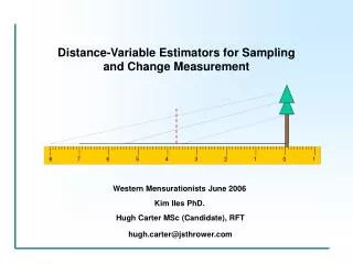
Distance-Variable Estimators for Sampling and Change Measurement 8 7 6 5 4 3 2 1 0 1 Western Mensurationists June 2006 Kim Iles PhD. Hugh Carter MSc (Candidate), RFT hugh.carter@jsthrower.com
8 0 7 1 6 2 5 3 4 4 3 5 2 6 7 1 8 0 9 1 Outline • Background • Bias (or lack of) • Shapes • Change over time • Compatibility • Simple example • Edge • Future Work • Summary
8 0 7 1 2 6 5 3 4 4 5 3 6 2 1 7 0 8 1 9 Background • A reminder of why we might want to use Variable Radius Plots • (VRP) for measuring change: • - Efficiency (cost and time). • - Remeasurement of existing plots. • - Increase precision? • Need a solution for applying VRP for measuring change over time. • Problems encountered include: • - High variability due to on-growth. • - Extending concepts to variables other than volume and BA. • - Providing a solution that is easily applied and understood.
8 0 7 1 2 6 5 3 4 4 5 3 6 2 1 7 0 8 1 9 Background Continued • Attempts have been made to solve these problems, however none • have covered them all. • Distance-Variable estimators reduce variability, extend to any • variable for any object of interest, and provide an easy to apply • method. • Distance-Variable estimators are an extension of the “Iles method” • to any variable of interest on any sampled object of interest.
8 0 7 1 6 2 5 3 4 4 3 5 2 6 1 7 0 8 1 9 Bias Horvitz-Thompson Estimator Potential random sample points Object of interest Inclusion circle
8 0 7 1 6 2 3 5 4 4 3 5 6 2 7 1 0 8 1 9 Expectation of Bias Continued Distance-Variable Estimator Potential random sample points Object of interest Inclusion circle
8 0 7 1 6 2 5 3 4 4 5 3 6 2 1 7 0 8 1 9 Shapes Why Use a Cone? 3x Value • Easy to use and visualize • - height at point is 3x value • - height at base is 0x value • Average at all potential sample • points will give estimate • Can get a simple “Value Gradient” 0x Value
8 0 7 1 2 6 3 5 4 4 5 3 2 6 7 1 0 8 1 9 Shapes Continued How do they work? 111 m2/s2/kg • Units no longer an issue • Average at sample points give estimate • Sample point is ¼ of distance from edge • Estimate = ¼ * 111m2/s2/kg = 27.37m2/s2/kg 0 m2/s2/kg Average of all sample points is 37 m2/s2/kg
0 8 1 7 2 6 5 3 4 4 5 3 6 2 7 1 0 8 1 9 Change Over Time Traditional Subtraction Method
0 8 1 7 2 6 5 3 4 4 5 3 6 2 7 1 0 8 1 9 Change Over Time Distance-Variable Method
0 8 1 7 2 6 3 5 4 4 5 3 6 2 7 1 8 0 1 9 Compatibility Both methods are compatible, however the traditional subtraction method is more variable!
8 0 1 7 2 6 5 3 4 4 3 5 6 2 1 7 8 0 1 9 Basal Area Example Traditional Method (BAF 10m2/ha) 40 35 Total 30 25 Total BA/ha 20 15 10 5 0 On-growth 0 1 2 3 4 Measurement Distance-Variable Method (BAF 10m2/ha) Survivor Total Mortality On-Growth On-growth
0 8 1 7 6 2 5 3 4 4 5 3 6 2 1 7 8 0 1 9 Basal Area Example Traditional Method (BAF 10m2/ha) Total Total Survivor Distance-Variable Method (BAF 10m2/ha) Survivor Total Mortality On-Growth Survivor
0 8 1 7 6 2 5 3 4 4 5 3 6 2 1 7 8 0 1 9 Basal Area Example Traditional Method (BAF 10m2/ha) Total Total Mortality Distance-Variable Method (BAF 10m2/ha) Survivor Total Mortality On-Growth Mortality
0 8 1 7 2 6 5 3 4 4 5 3 2 6 7 1 8 0 9 1 Basal Area Example Traditional Method (BAF 10m2/ha) Total Total Total Mortality Tree Survivor Tree On-Growth Tree Survivor On-growth Mortality Distance-Variable Method (BAF 10m2/ha) Survivor Tree Total Mortality Tree On-Growth Tree Survivor On-growth Mortality
8 0 7 1 6 2 5 3 4 4 5 3 6 2 1 7 0 8 1 9 Edge • Existing techniques for correcting edge remain applicable. - Walk-through - Toss-back - Mirage • Unbiased if inclusion areas are symmetrical through the tree. • If extra sample points are needed the DV estimator is used • instead of the traditional estimator.
8 0 7 1 6 2 5 3 4 4 3 5 2 6 1 7 0 8 1 9 Future Work • Variance control through different shaped estimators. • Non-stationary object sampling. • Density surface mapping. • Efficiency/Precision gains?
8 0 7 1 2 6 5 3 4 4 3 5 6 2 1 7 8 0 1 9 Summary Distance-Variable Method • EXTENDS TO ANY VARIABLE FOR ANY OBJECT!! • Unbiased • Easy to apply and understand • Smoothes change/growth curves • Compatible • Works with existing edge techniques
0 8 1 7 2 6 5 3 4 4 5 3 6 2 7 1 0 8 1 9 Acknowledgements Kim Iles & Associates
0 8 7 1 6 2 3 5 4 4 5 3 6 2 7 1 0 8 1 9 Volume Example Traditional Method Distance-Variable Method
8 0 7 1 6 2 5 3 4 4 3 5 2 6 7 1 8 0 9 1 Summary • Background • Bias (or lack of) • Shapes • Change over time • Compatibility • Simple example • Edge • Future Work • Summary