Download
1 / 16
170 likes | 301 Views
Sampling Distributions. Welcome to inference!!!! Chapter 9. Parameter. A Parameter is a number that describes the population. A parameter always exists but in practice we rarely know it’s value b/c of the difficulty in creating a census.

E N D
Sampling Distributions Welcome to inference!!!! Chapter 9
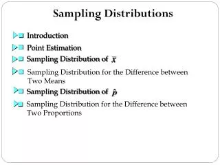
Parameter • A Parameter is a number that describes the population. • A parameter always exists but in practice we rarely know it’s value b/c of the difficulty in creating a census. • We use Greek letters to describe them (likeμorσ). If we are talking about a percentage parameter, we use rho (ρ) • Ex: If we wanted to compare the IQ’s of all American and Asian males it would be impossible, but it’s important to realize that μAmericans and μmales exist. • Ex: If we were interested in whether there is a greater percentage of women who eat broccoli than men, we want to know whether ρwomen > ρmen
Statistic • A statistic is a number that describes a sample. The value of a statistic can always be found when we take a sample . It’s important to realize that a statistic can change from sample to sample. • Statistics use variables like x bar, s, and phat (non greek). • We often use statistics to estimate an unknown parameter. • Ex: I take a random sample of 500 American males and find their IQ’s. We find that x bar = 103.2. • I take a random sample of 200 women and find that 40 like broccoli. Then phatw = .2 • IMPORTANT! A POPULATION NEEDS TO BE AT LEAST 10 TIMES AS BIG AS A SAMPLE TAKEN FROM IT. IF NOT, YOU NEED A SMALLER SAMPLE
Bias • We say something is biased if it is a poor predictor
Variability *Variability of population doesn’t change- (scoop example) size of scoop matters
How can we use samples to find parameters if they give us different results? • Imagine an archer shooting many arrows at a target: 4 situations can occur • a) consistent but off target. b) all over the place. tends to average a bulls eye but each result is far from center. c) worse than a as the archer is consistently missing high and to the right but nearly as consistently as situation a. d) is ideal- low bias and low variability.
Here’s an example: • Suppose our goal was to estimate μamericanmale. • We can’t take a census, so we take many samples. We find the average IQ of american males in each sample (x bar). • a) if our many samples of IQ’s are consistent but higher than the true average IQ of AM’s, then we have a situation with high bias and low variability • b) If our many samples are inconsistent- some high, some low than the true mean of AM’s Iqs, we have low bias and high variability.
If our sample means are not close to each other but all higher than μAM then we have high bias and high variability (c) • Finally, if our samples all just slightly higher or slightly lower than μAM, we have our desired situation: low bias and low variability.
But… • You aren’t taking a bunch of samples…you’re only going to take 1! and we want it to predict μam • If we used the data from situation d) then any of the samples would provide a good predictor for μam • We already know some ways to get a good sample- using an SRS and being very sure to have no bias when choosing our sample. • Inference is using our sample statistic (assuming it’s a good sample) to predict our parameter with a certain degree of confidence.
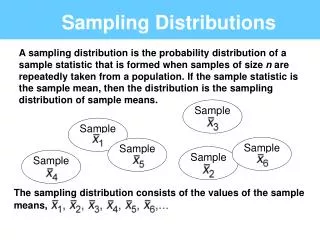
The Sampling Distribution • The sampling distribution of a statistic is the distribution of means of all possible samples of the same size from the population. • When we sample, we sample with replacement. • A sampling distribution is a sample space- it describes everything that can happen when we sample. Cool demo
Central Limit Theorem (CLT) • As you take more and more SRS’s of the same size, the distribution of their means will get closer and closer to a normal curve centered around the true population mean…NO MATTER WHAT THE SHAPE OF THE PARENT POPULATION!! Why?! • The Sampling Distribution of means has a mean of μand a standard deviation of σ/√n** N(μ,σ/√n)
CLT summary • 1. The mean of the population (what we want to find) will be the same as the mean of all your many samples. • 2. The Standard Deviation of all your many samples will be the population standard deviation divided by √n (your sample size) • 3. The histogram of the samples will appear normal (bell shaped). • 4. The larger the sample size (n), the smaller the standard deviation will be and the more constricted the graph will be.
What if we’re talking about proportions? • Same thing except we use our proportion formulas for mean and standard deviation
Don’t forget our rule of 10! • Only use σ/√n or if the 10 times N (the number of people in our population) is ≥ n (the number of people in our sample)
Example • The true average study time for a final exam in history is found to be 6 hours and 25 minutes with a standard deviation of 1 hour and 45 minutes. Assume the distribution is normal. N(6.417, 1.75) • What is the probability that a student chosen at random spends more than 7 hours studying? Normalcdf(7,100,6.417,1.75) = 37% • What is the probability that an SRS of 4 students will average more than 7 hours in studying? Normalcdf(7,100,6.417,1.75/√4) = 25.3%. • Why did the probability go down? • A student to study more than 7 hours is not probable…a group of 4 to average more than 7 is less probable.
Example 2 • The length of pregnancy from conception to birth varies normally with a mean of 266 days and a standard deviation of 16 days • N(266,16) • What is the probability that a woman chosen at random has a pregnancy lasting more than 270 days? • 40.1% • What is the mean and standard deviation of my sampling distribution? • What is the probability that an SRS of 16 women have pregnancies averaging more than 270 days?