Topic 3 - Digital Images
240 likes | 441 Views
Topic 3 - Digital Images. Department of Physics and Astronomy. DIGITAL IMAGE PROCESSING Course 3624. Professor Bob Warwick. 3.1 What is a Digital Image?.

Topic 3 - Digital Images
E N D
Presentation Transcript
Topic 3 - Digital Images Department of Physics and Astronomy DIGITAL IMAGE PROCESSING Course 3624 Professor Bob Warwick
3.1 What is a Digital Image? • An analogue image is a 2-dimensional (2-d) continuous light intensity distribution, , where x and y are spatial coordinates. • A digital image is a representation of the continuous (analogue) image by a 2-d array of numbers. • The digital image is obtained by sampling at points on a regular grid. The amplitude at each sampling point is quantized, and represented (initially) as a binary number. Notes: • After processing the digital image may be stored as a 2-d array of integers, real or complex numbers. • Each element of the 2-d array is a pixel (derived from “picture element”).
Analogue versus Digital Image Formats Analogue ImageDigital Image (M x N Pixels) y y’ (0,0) (0,Y) f00 f01 f10 f02 x x’ f20 fM-1,N-1 (X,0) (X,Y) Continuous variables x,y x = 0 X y = 0 Y Indices x’,y’ x' = 0,1,2 M-1 y' = 0,1,2 N-1
The two-step process Sampling on a M x N spatial grid: Cell size is: Δx = X/M Δy = Y/N Sampling points in x & y are: x= (x’ + 0.5) Δx y= (y’ + 0.5) Δy y’ 0 1 2 ……… 0 1 2 . . . x’
Quantization Step where p is an integer which defines the number of quantization levels, eg p = 8 implies 256 levels. Then assign: Rounded down to an integer value
Quantization Step 2p – 1 2p - 2 2 1 0 The exponent p corresponds to the number of bits in the Analogue-to-Digital conversion employed in the digitization. Notes: Hereafter = the "gray level" Range 0 2P-1 is known as the grayscale of the image
Construction of a Digital Colour Image A digital monochrome image consists of a 2-d array of numbers. A digital colour image consists of three such 2-d arrays (one for each component colour.
3.2 Information Loss in Digitization Quantization Step Noise is added equivalent to roughly 1/3 of an ADC step (ie 1 bit)
Information Loss in Spatial Sampling x The above depicts two sinusoidal signals in an input 1-d (analogue) image that fit the same set of sample values. If the input contains signals varying such that: signal rate > sampling rate/2 then information may be lost (as above). This problem is known as ALIASING – see topic 7.
3.3 Image Quality Considerations Whether an image is classed as of “good”, “moderate” or “poor” quality” is invariably a very subjective assessment, dependent to a large degree on the amount of detail in the scene. As a “rule-of-thumb” a grayscale image with: 512 x 512 pixels with 32 gray levels will be comparable to an old b/w TV picture. Nb 8 binary bits = 1 byte = 256 levels 1024 x 1024 x 1 byte 1 Megabyte (eg CPU memory) 1000 x 1000 x 1 byte 1 Megabyte (eg computer storage)* Eg. A high resolution digital camera recording 12 megapixel images in colour will generate files of 36 Mbytes /image (assuming 3 bytes per pixel). CPU Memory - 2-8 Gbytes (typically) CD ROMs - 0.6-0.9 Gbytes DVDs - 4.7 Gbytes Hard Disks - 1 Terabyte Human Brain - 125 Terabytes
Halftone Image Binary Image
3.4 Image File Formats and Image Compression Image file formatsare standardized means of organizing and storing digital images. They consist of "header information" followed by the "image data". The different image file formats apply a variety ofimage file compressionalgorithms to reduce the image file size for storage: Lossless compressionalgorithms reduce file size without losing information (ie are error-free) - used when image integrity is valued above file size (eg scientific data). Lossy compressionalgorithms take advantage of the inherent limitations of the human eye and discard "redundant" information. Most lossy compression algorithms allow for a variable quality level and compression ratio. As the latter is increased, file size is reduced. At the highest compression levels, when the image is decompressed (ie reconstructed), image deterioration becomes noticeable as "compression artefacting”.
Some Popular Image File Formats JPG/JPEG (Joint Photographic Experts Group) is a compression method which (in most cases) is lossy. Nearly every digital camera can save images in JPEG format. It supports 8-bits per colour. The compression ratio is selectable. GIF (Graphics Interchange Format) is limited to an 8-bit palette, or 256 colors. This makes the GIF format suitable for storing graphics with relatively few colours such as simple diagrams, shapes, logos and cartoon style image. It also supports animation. It uses a lossless compression that is most effective when large areas have a single colour, and ineffective for detailed images. FITS (Flexible Image Transport System) is often used for scientific applications. It stores the original (image) data in a structured way.
Effects of JPEG Compression Maximum quality 38384 bytes High quality 11331 bytes Medium quality 6968 bytes Low quality 5141 bytes Low quality 1554 bytes Low quality 3687 bytes