Download
1 / 76
760 likes | 900 Views
Singa and kappa analyses at BESII. Ning Wu Institute of High Energy Physics, CAS Beijing, China January 25-26, 2007. Introduction.

E N D
Singa and kappa analyses at BESII Ning Wu Institute of High Energy Physics, CAS Beijing, China January 25-26, 2007
Introduction • The existence of and had been suggested from various viewpints both theoretically and phenomenologically. Early analysis of I=0 S-wave phase shift make the conclusions against the existence of the σ particle. As a results, it had ever disappeared from PDG for about 20 years. But most re-analysis of ππ/πK scattering data support the existence of the and particles. • In early studies, most evidences of the existence of and come from ππ/πK scattering. If and particles exist, they should also be seen in the production processes. Searching and studying and in production processes is also important for us to know their properties and structures.
Introduction(2) • We first found evidence of the existence of σand κparticles in 7.8M BESI J/ψdata. After BESII obtain much larger J/ψdata sample, we moved our analysis to be based on BESII data. • Based on BES J/ψ decay data, a low mass enhancement in ππ spectrum in J/ψωππ and a low mass enhancement in Kπ spectrum in J/ψK*(892)Kπ are found. In order to prove that they are σand κparticles, we need not only to measure their pole positions, but also to determine their spin-parity. So, PWA analyses are needed to study σand κparticles in these two channels.
Introduction(3) • PWA analysis is widely used in BES physics analysis in past a few years. It is used to determine mass, width and branching ratio of a resonance, and to determine its spin-parity. • In this talk, we discuss PWA analyses of J/ψωππ and J/ψK*(892)K. • Main contents of the talk are • Helicity Formalism • Maximum Likelihood Method • PWA analysis on J/ψωππ • PWA analysis on ψ′ππJ/ψ • PWA analysis on J/ψK*(892)K • Summary
Helicity Formalism • For a two-body decay process a b + c spin J sb sc momentum pa pb pc helicity m λb λc parity a b c • Its S-matrix element is Reltive momentum of two final state particles in center of mass syetem
Helicity Formalism(2) • The decay amplitude is D-function Helicity coupling amplitude All angular information of the decay vertex are contained in the D-function, and helicity coupling amplitude is independent of all angular variables.
Helicity Formalism(3) • In J/ψhadronic or radiative decay processes, parity conservation is hold. The heliclity coupling amplitude has the following symmetry • If two final state particle b and c are identical particles, the wave function of final state system should be symmetric or antisymmetric, and
Helicity Formalism(4) • In experimental physics analysis, most decays we encountered are sequential decays, and resonant states appear as intermediate states. • The decay amplitude for this sequential decay is c a d b e Decay amplitude for ab+c Breit-Wigner function of the resonance b Decay amplitude for bd+e
Maximum Likelihood Method • In experimental physics analysis, after we obtain a data sample, we first need to know how many resonances appear and what is the decay mechanism. Then we need to calculate the differential cross-section =(1,2,…) helicities of final state particles =(1,2,…) helicities of intermediate resonances m helicity of the mother particle dΦ element of phase space BG non-interference backgrounds i components considered
Maximum Likelihood Method(2) • Normalized probability density function which is used to describe the whole decay process is σ total cross section W(Φ) effects of detection efficiency x quantities which are measured by experiments α unknown parameters which need to be determined in the PWA fit.
Maximum Likelihood Method(3) • Total cross-section is defined by NMC the total number of Monte Carlo events ( … )j the quantity is calculated from the j-th Monte Carlo events • It is required that these Monte Carlo events are obtained through real detection simulation and have passed all cut conditions which are used to to obtain the data sample of the process.
Maximum Likelihood Method(4) • The maximum likelihood function is given by the adjoint probability for all the data • Define • In the data analysis, the goal is to find the set of unknown parameters α by minimizing S. Mass and width of a resonance are determined by mass and width scan. Spin-parity of a resonance is determined by comparing fit quality with different solution of different spin-parity.
Study of Particle at BES • Clear signals of σ particle are found in two channels at BES: • J/ψ→ωππ • Ψ′→ππJ/ψ
Pole in J/ψ→ωπ+π- • This channel was ever studied by MARKIII, DM2 and BES. • In the early studies, the low mass enhancement does not obtain enough attention. • Since 2000, BES had performed careful study on the structure of the low mass enhancement, and measured parameters of its pole position. • Data sample: BESI 7.8M J/ψ events • BESII 58M J/ψ events
Study of σ Based on 58M BESII J/ψ Events π0 and ω Signal BESII
BESI Invariant mass spectrum and Daliz plot BESI BESII BESII
Backgrounds Phase space effect Threshold Effects Resonance Possible Origin of the low mass enhancement
Background Study • Two different kinds of backgrounds • Contain ωparticle in the decay sequence: J/ψωX • Do not contain ωparticle in the decay sequence ω side-band does not contain the low mass enhancement, so it does not come from the second kind of backgrounds. After side-band subtraction BESII
Background Study Monte Carlo simulation of some J/ψ decay channels. All these backgrounds can not produced the low mass enhancement, so it can not also come from the first kind of backgrounds.
Backgound Study Generate 50M J/ψ anything Monte Carlo events. The generator is based on Lund-Charm model. It contain almost all known J/ψ decay channels. It contains the backgrounds of inclusive J/ψ decays.
Phase Space Effect Enents are not unifromly scattered in the whole phase space, the shape of the low mass enhancement is also different from that of phase space. Not a phase space effect. BESII
Threshold Effect A clear peak is seen in the phase space and efficiency corrected spectrum. Threshold effect should decrease monotonically at the threshold. BESII
Summary on σ origin • Not from backgrounds • Not a phase space effect • Not threshold effect • It should be a resonance
PWA Analysis • Two Independent PWA analysis are performed: • Using the method of relativistic helicity coupling amplitude analysis to analyze the spectrum of lower mass region • Using the Zemach formalism to analyze the spectrum of the whole mass region. • Results obtained from two independent analysis are basically consistent.
PWA analysis:0-1.5 GeV To avoid complicity in the higher mass region, and concentrate our study on the low mass enhancement, PWA analysis is performed only on the 0 — 1.5 GeV mass region. BESII
Components • The following components are considered: • σ • f2(1270) • f0(980) • b1(1235) • Background
PWA Analysis • The dominant backgrounds are phase space backgrounds and ρ3π backgrounds。 • Three different methods are used to fit BG.(free fit, directly side-band subtraction, fix BG to different level) • Large uncertainties comes from the fit on backgrounds, which is the main sources of uncertainties.
Spin-Parity 0++ Angular distributions of the low mass enhancement 2++ 4++
Spin-Parity Compare the fit quality
Parametrizations Constant width There does not exist a mature method to parametrize a wide resonance near threshold, so different parametrizations are tried in the fit. With contains ρ(s) Zheng’s parametrization
Mass, width and pole positions Three different parametrizations are used in this fit. Mass and width are obtained through the fit, pole positions are calculated theoretically. Eq.(9) BW of constant width Eq.(13) BW of width contains ρ Eq.(14) Zheng’s parametrization
Fit on the angular distributions of the lower mass region A 0++ resonance is used to fit σ particle.
Method II Another independent PWA analysis is performed in this channel. It analyze the whole mass region and the following processes are added into the fit.
Method II (continued) The σ particle is also needed in the fit of the low mass enhancement. The dominant contribution of the low mass enhancement also comes from the σ particle.
Method II (continued) Pole positions of the σ particle obtained by this method is consistent with above. The combined results are (541±39) –i (252±42) MeV. With ρ Constant
σ particle in Ψ′→ππJ/ψ • The ππ mass spectrum can be fit phenomenonlogically. • It can also be fit by σ particle destructively interfere with a broad scalar structure, i.e. |BW(σ)+IPS|2.
σ particle in Ψ’→ππJ/ψ Three different BW parametrizations are also tried in the fit. The shape of the BW given by different parametrizations are almost the same. Strong destructive interference, so that the amplitude at threshold is almost zero.
σ particle in Ψ’→ππJ/ψ • Different parametrizations are tried in the PWA fit. • Results on pole positions given by these parametrizations are quite consistent.
Summary on σ pole positions BESI J/ψ data BESII J/ψ data ωππ system BESII J/ψ data 5π system BESII ψ′ data
Study of κ Particle at BES Clear signal of κ particle is found in the Kπ invariant mass spectrum in the decay channel J/ψ→K*(892)0Kπ. It is seen at both BESI and BESII data.
κ particle in J/ψ→K*(892)0K+π- For our BESII data, the statistics are much larger. BESII data
Recoil mass spectrum against K*(892)0 κ signal is clear in the invariant mass spectrum.
Dalitz Plot κ signal is clear in the Dalitz plot.
Charge conjugate channel The spectrum is almost the same as that of the charge conjugate channel.
Possible origin • Backgrounds • Phase space effects • Threshold effects • Resonance
Background Study K*(892)0 side-band