Forecasting
350 likes | 800 Views
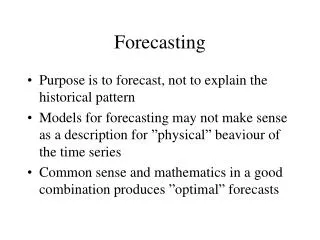
Forecasting. Purpose is to forecast, not to explain the historical pattern Models for forecasting may not make sense as a description for ”physical” beaviour of the time series Common sense and mathematics in a good combination produces ”optimal” forecasts.

Forecasting
E N D
Presentation Transcript
Forecasting • Purpose is to forecast, not to explain the historical pattern • Models for forecasting may not make sense as a description for ”physical” beaviour of the time series • Common sense and mathematics in a good combination produces ”optimal” forecasts
With time series regression models, forecasting (prediction) is a natural step and forecasting limits (intervals) can be constructed • With Classical decomposition, forecasting may be done, but estimation of accuracy lacks and no forecasting limits are produced • Classical decomposition is usually combined with Exponential smoothing methods
Exponential smoothing • Use the historical data to forecast the future • Let different parts of the history have different impact on the forecasts • Forecast model is not developed from any statistical theory
Single exponential smoothing • Assume historical values y1,y2,…yT • Assume data contains no trend, i.e.
Forecasting scheme: where is a smoothing parameter between 0 and 1
The forecast procedure is a recursion formula • How shall we choose α? • Where should we start, i.e. Which is the initial value l0 ?
Use a part (usually half) of the historical data to estimate β0 Set l 0= Update the estimates of β0 for the rest of the historical data with the recursion formula l Twhich can be used to forecastyT+τ
Example: Sales of everyday commodities Year Sales values 1985 151 1986 151 1987 147 1988 149 1989 146 1990 142 1991 143 1992 145 1993 141 1994 143 1995 145 1996 138 1997 147 1998 151 1999 148 2000 148
Assume the model: Estimate β0by calculating the mean value of the first 8 observations of the series Set l8 = =146.75
Assume first that the sales are very stable, i.e. during the period the mean value β0 is assumed not to change Set α to be relatively small. This means that the latest observation plays a less role than the history in the forecasts. Thumb rule: 0.05 < α < 0.3 E.g. Set α=0.1 Update the estimates of β0using the next 8 values of the historical data
Alternative In Bowerman/O’Connell/Koehler the updates of estimates of β0are done on all historical data i.e. for T=1,…, n and l0=
MTB > Name c3 "FORE1" c4 "UPPE1" c5 "LOWE1" MTB > SES 'Sales values'; SUBC> Weight 0.1; SUBC> Initial 8; SUBC> Forecasts 3; SUBC> Fstore 'FORE1'; SUBC> Upper 'UPPE1'; SUBC> Lower 'LOWE1'; SUBC> Title "SES alpha=0.1". Single Exponential Smoothing for Sales values Data Sales values Length 16 Smoothing Constant Alpha 0.1
Accuracy Measures MAPE 2.2378 MAD 3.2447 MSD 14.4781 Forecasts Period Forecast Lower Upper 17 146.043 138.094 153.992 18 146.043 138.094 153.992 19 146.043 138.094 153.992
Assume now that the sales are less stable, i.e. during the period the mean value β0 is possibly changing Set α to be relatively large. This means that the latest observation becomes more important in the forecasts. E.g. Set α=0.5 (A bit exaggerated)
Single Exponential Smoothing for Sales values Data Sales values Length 16 Smoothing Constant Alpha 0.5 Accuracy Measures MAPE 1.9924 MAD 2.8992 MSD 13.0928 Forecasts Period Forecast Lower Upper 17 147.873 140.770 154.976 18 147.873 140.770 154.976 19 147.873 140.770 154.976
We can also use some adaptive procedure to continuosly evaluate the forecast ability and maybe change the smoothing parameter over time Alt. We can run the process with different alphas and choose the one that performs best. This can be done with the MINITAB procedure.
Single Exponential Smoothing for Sales values --- Smoothing Constant Alpha 0.567101 Accuracy Measures MAPE 1.7914 MAD 2.5940 MSD 12.1632 Forecasts Period Forecast Lower Upper 17 148.013 141.658 154.369 18 148.013 141.658 154.369 19 148.013 141.658 154.369 Yet, wider prediction intervals
Exponential smoothing for times series with trend and/or seasonal variation • Double exponential smoothing (one smoothing parameter) for trend • Holt’s method (two smoothing parameters) for trend • Multiplicative Winter’s method (three smoothing parameters) for seasonal (and trend) • Additive Winter’s method (three smoothing parameters) for seasonal (and trend)
Example: Real Estate Price Index for Weekend Cottages in Sweden Year REPI_C 1993 226 1994 241 1995 239 1996 240 1997 268 1998 303 1999 336 2000 414 2001 472 2002 496 2003 505 2004 546 2005 591 Trend but no seasonal variation
Applying Holt’s method with MINITAB (denoted Double exponential smoothing in Minitab)
2 smoothing parameters, one for level and one for trend. Option to let Minitab calculate optimal parameters. Smoothing parameters should still be kept low (0.05,0.3)
Double Exponential Smoothing for REPI_C Data REPI_C Length 13 Smoothing Constants Alpha (level) 0.2 Gamma (trend) 0.2 Accuracy Measures MAPE 9.78 MAD 30.15 MSD 1160.79 Forecasts Period Forecast Lower Upper 14 611.411 537.537 685.286 15 646.167 570.753 721.581
Example: Quarterly sales data year quarter sales 1991 1 124 1991 2 157 1991 3 163 1991 4 126 1992 1 119 1992 2 163 1992 3 176 1992 4 127 1993 1 126 1993 2 160 1993 3 181 1993 4 121 1994 1 131 1994 2 168 1994 3 189 1994 4 134 1995 1 133 1995 2 167 1995 3 195 1995 4 131
3 smoothing parameters, one for level, one for trend an one for seasonal variation. No option to calculate optimal parameters. Choices have do be based on visual inspection of the times series
Winters' Method for sales Multiplicative Method Data sales Length 20 Smoothing Constants Alpha (level) 0.2 Gamma (trend) 0.2 Delta (seasonal) 0.2 Accuracy Measures MAPE 2.6446 MAD 3.8808 MSD 23.7076 Forecasts Period Forecast Lower Upper Q3-2013 135.625 126.117 145.133 Q4-2013 174.430 164.773 184.087 Q1-2014 194.667 184.844 204.490 Q2-2014 136.933 126.928 146.939