Download
1 / 24
240 likes | 438 Views
Using GC content to distinguish Phytophthora sequences from tomato sequences. Mission #1. Calculate the GC content of each sequence in the Phytophthora -tomato interactome We will use a perl script to accomplish the mission. Preparation.

E N D
Using GC content to distinguish Phytophthora sequences from tomato sequences
Mission #1 Calculate the GC content of each sequence in the Phytophthora-tomato interactome We will use a perl script to accomplish the mission.
Preparation • Download the perl script (gc.pl) from the class web site and store it in C:/BioDownload folder
Running the script • Open cygwin, or command prompt (Vista users), or terminal (Mac users) • Change directory (cd) to the BioDownload folder • perl<space>gc.pl<space>PhytophSeq1.txt<space>phyto_gc.out
Results In cygwin (Windows users) or terminal (Mac users) grep<space>--perl-regexp<space>”\t”<space>-c<space>phytoph_gc.out grep<space>”>”<space>-c<space>PhytophSeq1.txt You should get the same number from the two commands. The number should be 3921.
The output file Name column GC content column
Mission #2 Build a histogram of the values of GC content We will use R program to accomplish this mission.
XP users Vista users
setwd(“c:/BioDownload”) to change the working directory to C:/BioDownload setwd(“/path/to/biodownload”) for Mac users
data<-read.table(“phytoph_gc.out”,sep=“\t”,header=FALSE)data<-read.table(“phytoph_gc.out”,sep=“\t”,header=FALSE) to read in the data in the file phytoph_gc.out (your file name may be different)
data[1:10,] to see the first 10 lines of the vector “data”
gc<-data[,2] to assign the values from the 2nd column of “data” to a new vector “gc”
summary(gc) to get the summary of the values in the vector “gc”
hist(gc,breaks=58) to draw a histogram of the values in “gc” vector Breaks indicates how many cells you want for the histogram. It was calculated as 78.7 (max) - 21.2 (min). It means the bin of the histogram is ~ 1 GC value
hist(gc,breaks=58,xlab=“GC content”,ylim=range(c(0,400)),main=“Histogram of GC content of sequences\ninPhytophthora-tomato interactome”) to make the histogram look better
>pdf(“gc_histogram.pdf”) >hist(gc,breaks=58,xlab=“GC content”,ylim=range(c(0,400)),main=“Histogram of GC content of sequences\ninPhytophthora-tomato interactome”) >dev.off() To output the histogram to a PDF file.
location file