Understanding Dissolved Oxygen Dynamics in Lakes: A Multi-Scale Analysis
This study examines the control mechanisms of dissolved oxygen (DO) across various lakes using wavelet transforms to analyze ecological data. We assess the effects of light and wind on DO levels, tracking changes over different scales and identifying relationships with gross primary productivity (GPP) and respiration rates. By employing advanced statistical models, including AIC for model selection, we explore variability in DO across diverse environmental conditions, contributing to a deeper understanding of aquatic ecosystems.

Understanding Dissolved Oxygen Dynamics in Lakes: A Multi-Scale Analysis
E N D
Presentation Transcript
The Projects • Control of DO across scales • Langman et al. • Beyond Odum • Hanson et al. • Surprise! • Langman et al.
Unprocessed Data Hummingbird Trout Bog Allequash Source: Owen Langman
Single Lake Wavelet Decompositions Wavelet Transforms: A method of separating a signal into frequency components while preserving the time domain. Continuous Wavelet Transforms: A signal of finite length and energy is projected on a continuous family of frequency bands. Trout Bog; 24+ hr; DO, T Hummingbird; 2 hr; DO, U Allequash; 24 hr; DO, I Source: Owen Langman
The effect of light on DO 30 25 20 15 10 5 1 Scale (hr) Lake area (ha) Source: Owen Langman
The effect of wind on DO 30 25 20 15 10 5 1 Scale (hr) Lake area (ha) Source: Owen Langman
P, Tair, U PAR Crystal Bog Dissolved Oxygen (mg/L) dO2/dt = GPP – R – Fatm + A (Odum 1956) MetDataWoodruffAirport.xls
Pmax GPP = Pmax.* (1- exp(-IP * I / Pmax)) IP IR R0 (night time R) Simple model Complicated model(s) Gross Primary Productivity, Respiration P0 (always= 0) 0 0 Irradiance Figure X. Responses for ecosystem GPP and R as a function of irradiance. Parameters are per Table X.
Test of the Ibeta (light history) parameter I original Beta = 0.1 Beta = 1 Beta = 10 Beta = 100 Effective I Time of day RunSimulation.m
Processes: Night R GPP GPP Day R Light history • Use simulated data to determine which are identifiable. • Fit all the valid models for 3 lakes over one week. • Use AIC to discriminate among models.
GPP R NEP Fatm Crystal Bog Irradiance • Models performed similarly • Biology explains diel • Much unexplained variability • Fatm similar to NEP DO observations, models (mg/L) Processes Day fraction GraphResults.m
GPP R NEP Fatm Trout Bog Irradiance • Midnight surge unexplained • Complex model best • Fatm similar to NEP DO observations, models (mg/L) Processes Day fraction GraphResults.m
GPP R NEP Fatm Trout Lake Irradiance • Complex model best • NEP >> Fatm • R remains elevated DO observations, models (mg/L) Processes Day fraction GraphResults.m
Sparkling L. 2004 1-6 m Temperature (C)
Surprise Theory Posterior PDF Prior PDF Kullback-Leibler divergence measures the difference between the distributions • Result: A quantitative single value measuring how unexpected the point is based on the amount of change from the prior to the posterior • Prior can be formed from historical data, existing models, or developed over a short training period from real time data • Capable of observing events at multiple temporal scales • Capable of observing events in 2D / 3D space Source: Owen Langman
Table X. AIC scores for each model for each lake. Model with the lowest AIC has the rank of 1. CompareModels.m => ResultsSummary.xls
% Parameter sets ************************************ Parameters = [0 3.0 0.005 0.001 5 20 0.1]; % PO RO IP IR Pmax Ibeta Physics InitialDO = 7.5; Sigma = 0.1 mg L-1 d-1 Sigma = 1.0mg L-1 d-1 DO (mg L-1) Sigma = 20mg L-1 d-1 Day fraction